from d2l import torch as d2l
import torch
from torch import nn6.4 Multiple Input and Multiple Output Channels
The single-channel operator of Section 6.2 cannot yet combine the red, green, and blue measurements of an image, nor can it produce several learned feature maps. With \(c_\textrm{i}\) input channels, an input has shape \(c_\textrm{i}\times h\times w\) and each filter has one spatial kernel per input channel. Producing \(c_\textrm{o}\) features requires \(c_\textrm{o}\) such filters, so the complete kernel has shape \(c_\textrm{o}\times c_\textrm{i}\times k_\textrm{h}\times k_\textrm{w}\). This section derives both channel operations and then factorizes the dense kernel to reduce its cost.
from d2l import tensorflow as d2l
import tensorflow as tf
from d2l import jax as d2l
from flax import nnx
import jax
from jax import numpy as jnpfrom d2l import mxnet as d2l
from mxnet import np, npx
from mxnet.gluon import nn
npx.set_np()6.4.1 Multiple Input Channels
When the input data contains multiple channels, we need to construct a convolution kernel with the same number of input channels as the input data, so that it can perform cross-correlation with the input data. Assuming that the number of channels for the input data is \(c_\textrm{i}\), the number of input channels of the convolution kernel also needs to be \(c_\textrm{i}\). If our convolution kernel’s window shape is \(k_\textrm{h}\times k_\textrm{w}\), then, when \(c_\textrm{i}=1\), the convolution kernel is a two-dimensional tensor of shape \(k_\textrm{h}\times k_\textrm{w}\).
However, when \(c_\textrm{i}>1\), we need a kernel that contains a tensor of shape \(k_\textrm{h}\times k_\textrm{w}\) for every input channel. Concatenating these \(c_\textrm{i}\) tensors together yields a convolution kernel of shape \(c_\textrm{i}\times k_\textrm{h}\times k_\textrm{w}\). Since the input and convolution kernel each have \(c_\textrm{i}\) channels, we can perform a cross-correlation operation on the two-dimensional tensor of the input and the two-dimensional tensor of the convolution kernel for each channel, adding the \(c_\textrm{i}\) results together (summing over the channels) to yield a two-dimensional tensor. This is the result of a two-dimensional cross-correlation between a multi-channel input and a multi-input-channel convolution kernel.
Figure 6.4.1 provides an example of a two-dimensional cross-correlation with two input channels. The shaded portions are the first output element as well as the input and kernel tensor elements used for the output computation: \((1\times1+2\times2+4\times3+5\times4)+(0\times0+1\times1+3\times2+4\times3)=56\).
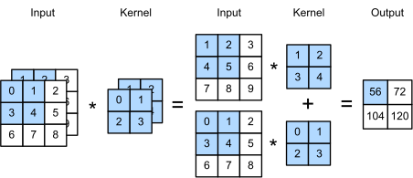
We can implement the multi-input-channel operation directly by computing one cross-correlation per channel and summing the results.
def corr2d_multi_in(X, K):
    # Iterate through the 0th dimension (channel) of K first, then add them up
    return sum(d2l.corr2d(x, k) for x, k in zip(X, K))
def corr2d_multi_in(X, K):
# Iterate through the 0th dimension (channel) of K first, then add them up
return tf.reduce_sum([d2l.corr2d(x, k) for x, k in zip(X, K)], axis=0)def corr2d_multi_in(X, K):
# Iterate through the 0th dimension (channel) of K first, then add them up
return sum(d2l.corr2d(x, k) for x, k in zip(X, K))def corr2d_multi_in(X, K):
# Iterate through the 0th dimension (channel) of K first, then add them up
return sum(d2l.corr2d(x, k) for x, k in zip(X, K))We can construct the input tensor X and the kernel tensor K corresponding to the values in Figure 6.4.1 to validate the output of the cross-correlation operation.
X = d2l.tensor([[[0.0, 1.0, 2.0], [3.0, 4.0, 5.0], [6.0, 7.0, 8.0]],
               [[1.0, 2.0, 3.0], [4.0, 5.0, 6.0], [7.0, 8.0, 9.0]]])
K = d2l.tensor([[[0.0, 1.0], [2.0, 3.0]], [[1.0, 2.0], [3.0, 4.0]]])

corr2d_multi_in(X, K)tensor([[ 56., 72.],
[104., 120.]])<tf.Tensor: shape=(2, 2), dtype=float32, numpy=
array([[ 56., 72.],
[104., 120.]], dtype=float32)>Array([[ 56., 72.],
[104., 120.]], dtype=float32)array([[ 56., 72.],
[104., 120.]])6.4.2 Multiple Output Channels
Regardless of the number of input channels, so far we always ended up with one output channel. However, as we discussed in Section 6.1.4, multiple channels are needed to represent different learned features. Many neural network architectures increase the channel dimension as we go deeper in the neural network, typically downsampling to trade off spatial resolution for greater channel depth. Each channel can respond to a different combination of features, but channels are optimized jointly rather than independently. An edge detector, for example, may correspond to a direction in channel space rather than to one channel.
Denote by \(c_\textrm{i}\) and \(c_\textrm{o}\) the number of input and output channels, respectively, and by \(k_\textrm{h}\) and \(k_\textrm{w}\) the height and width of the kernel. To get an output with multiple channels, we can create a kernel tensor of shape \(c_\textrm{i}\times k_\textrm{h}\times k_\textrm{w}\) for every output channel. We concatenate them on the output channel dimension, so that the shape of the convolution kernel is \(c_\textrm{o}\times c_\textrm{i}\times k_\textrm{h}\times k_\textrm{w}\). In cross-correlation operations, the result on each output channel comes from the convolution kernel corresponding to that output channel and draws on all channels in the input tensor.
We implement a cross-correlation function to calculate the output of multiple channels as shown below.
def corr2d_multi_in_out(X, K):
    # Iterate through the 0th dimension of K, and each time, perform
    # cross-correlation operations with input X. All of the results are
    # stacked together
    return d2l.stack([corr2d_multi_in(X, k) for k in K], 0)
We construct an illustrative convolution kernel with three output channels by concatenating the kernel tensor for K with K+1 and K+2.
K = d2l.stack((K, K + 1, K + 2), 0)
K.shapetorch.Size([3, 2, 2, 2])TensorShape([3, 2, 2, 2])(3, 2, 2, 2)(3, 2, 2, 2)Below, we perform cross-correlation operations on the input tensor X with the kernel tensor K. Now the output contains three channels. The result of the first channel is consistent with the result of the previous input tensor X and the multi-input channel, single-output channel kernel.
corr2d_multi_in_out(X, K)tensor([[[ 56., 72.],
[104., 120.]],
[[ 76., 100.],
[148., 172.]],
[[ 96., 128.],
[192., 224.]]])<tf.Tensor: shape=(3, 2, 2), dtype=float32, numpy=
array([[[ 56., 72.],
[104., 120.]],
[[ 76., 100.],
[148., 172.]],
[[ 96., 128.],
[192., 224.]]], dtype=float32)>Array([[[ 56., 72.],
[104., 120.]],
[[ 76., 100.],
[148., 172.]],
[[ 96., 128.],
[192., 224.]]], dtype=float32)array([[[ 56., 72.],
[104., 120.]],
[[ 76., 100.],
[148., 172.]],
[[ 96., 128.],
[192., 224.]]])6.4.3 \(1\times 1\) Convolutional Layer
A \(1 \times 1\) convolution, where \(k_\textrm{h} = k_\textrm{w} = 1\), does not combine adjacent pixels. It instead mixes channels independently at every spatial position and is widely used in deep networks (Lin et al. 2013; Szegedy et al. 2017).
Because the minimum window is used, the \(1\times 1\) convolution loses the ability of larger convolutional layers to recognize patterns consisting of interactions among adjacent elements in the height and width dimensions. The only computation of the \(1\times 1\) convolution occurs on the channel dimension.
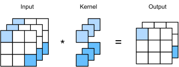
Figure 6.4.2 shows the cross-correlation computation using the \(1\times 1\) convolution kernel with 3 input channels and 2 output channels. The inputs and outputs have the same height and width. Each element in the output is derived from a linear combination of elements at the same position in the input image. You could think of the \(1\times 1\) convolutional layer as constituting a fully connected layer applied at every single pixel location to transform the \(c_\textrm{i}\) corresponding input values into \(c_\textrm{o}\) output values. Because this is still a convolutional layer, the weights are tied across pixel location. Thus the \(1\times 1\) convolutional layer requires \(c_\textrm{o}\times c_\textrm{i}\) weights (plus the bias). When a nonlinearity follows the layer, the \(1 \times 1\) convolution cannot in general be folded into an adjacent convolution.
We verify the equivalence by implementing a \(1 \times 1\) convolution using a fully connected layer. The only thing is that we need to make some adjustments to the data shape before and after the matrix multiplication.
def corr2d_multi_in_out_1x1(X, K):
    c_i, h, w = X.shape
    c_o = K.shape[0]
    X = d2l.reshape(X, (c_i, h * w))
    K = d2l.reshape(K, (c_o, c_i))
    # Matrix multiplication in the fully connected layer
    Y = d2l.matmul(K, X)
    return d2l.reshape(Y, (c_o, h, w))
When performing \(1\times 1\) convolutions, the above function is equivalent to the previously implemented cross-correlation function corr2d_multi_in_out. Let’s check this with some sample data.
X = d2l.normal(0, 1, (3, 3, 3))
K = d2l.normal(0, 1, (2, 3, 1, 1))
Y1 = corr2d_multi_in_out_1x1(X, K)
Y2 = corr2d_multi_in_out(X, K)
assert float(d2l.reduce_sum(d2l.abs(Y1 - Y2))) < 1e-5
X = d2l.normal((3, 3, 3), 0, 1)
K = d2l.normal((2, 3, 1, 1), 0, 1)
Y1 = corr2d_multi_in_out_1x1(X, K)
Y2 = corr2d_multi_in_out(X, K)
assert float(d2l.reduce_sum(d2l.abs(Y1 - Y2))) < 1e-5X = jax.random.normal(d2l.get_key(), (3, 3, 3))
K = jax.random.normal(d2l.get_key(), (2, 3, 1, 1))
Y1 = corr2d_multi_in_out_1x1(X, K)
Y2 = corr2d_multi_in_out(X, K)
assert float(d2l.reduce_sum(d2l.abs(Y1 - Y2))) < 1e-5X = d2l.normal(0, 1, (3, 3, 3))
K = d2l.normal(0, 1, (2, 3, 1, 1))
Y1 = corr2d_multi_in_out_1x1(X, K)
Y2 = corr2d_multi_in_out(X, K)
assert float(d2l.reduce_sum(d2l.abs(Y1 - Y2))) < 1e-56.4.4 Grouped, Depthwise, and Depthwise-Separable Convolutions
So far every output channel has depended on every input channel: the kernel carries \(c_\textrm{o} \times c_\textrm{i} \times k_\textrm{h} \times k_\textrm{w}\) weights, and both parameters and compute scale with the product \(c_\textrm{i} \cdot c_\textrm{o}\). A grouped convolution relaxes this. Split the \(c_\textrm{i}\) input channels into \(g\) groups of \(c_\textrm{i}/g\) channels each, split the \(c_\textrm{o}\) output channels likewise, and let each output group convolve over its own input group only. Viewed as a map on channels, the kernel becomes block-diagonal: \(g\) independent blocks of size \((c_\textrm{o}/g) \times (c_\textrm{i}/g)\) replace the single dense \(c_\textrm{o} \times c_\textrm{i}\) pattern of connections. The parameter and operation count drops from \(c_\textrm{i} c_\textrm{o} k_\textrm{h} k_\textrm{w}\) to \(g \cdot (c_\textrm{i}/g)(c_\textrm{o}/g) k_\textrm{h} k_\textrm{w} = c_\textrm{i} c_\textrm{o} k_\textrm{h} k_\textrm{w} / g\), a factor of \(g\). The price is that no information flows between groups within the layer, so architectures built on grouped convolutions restore the exchange elsewhere, typically with \(1\times 1\) convolutions between grouped layers. ResNeXt (Section 7.4.5) turns exactly this trade-off into a design principle.
Pushing the idea to its extreme, \(g = c_\textrm{i} = c_\textrm{o}\), gives the depthwise convolution: each channel is filtered by its own \(k_\textrm{h} \times k_\textrm{w}\) kernel and no channel mixing happens at all. This is the mirror image of the \(1\times 1\) convolution from Section 6.4.3, which mixes channels but ignores spatial structure. Composing the two, a depthwise \(k \times k\) convolution followed by a pointwise \(1\times 1\) convolution, yields the depthwise-separable convolution (Chollet 2017; Howard et al. 2017). Figure 6.4.3 contrasts it with the dense layer it replaces: the depthwise stage looks at neighborhoods within each channel, the pointwise stage recombines channels at each position.
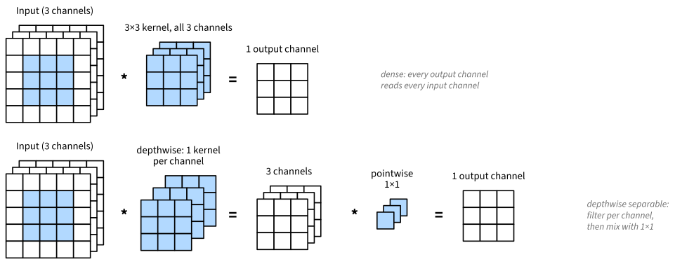
How much does the factorization save? For a \(k \times k\) kernel producing an \(h \times w\) output, the dense convolution costs \(h w \cdot c_\textrm{i} c_\textrm{o} k^2\) multiplications. The separable pair costs \(h w \cdot c_\textrm{i} k^2\) for the depthwise stage plus \(h w \cdot c_\textrm{i} c_\textrm{o}\) for the pointwise stage. The ratio is
\[ \frac{h w \cdot c_\textrm{i} k^2 + h w \cdot c_\textrm{i} c_\textrm{o}}{h w \cdot c_\textrm{i} c_\textrm{o} k^2} = \frac{1}{c_\textrm{o}} + \frac{1}{k^2}. \tag{6.4.1}\]
For \(k = 3\) and a large number of output channels this is close to \(1/9\): the separable layer is roughly eight to nine times cheaper, in parameters and in operations alike. This saving restricts expressivity. A depthwise-separable layer can only express convolutions that factor into a per-channel spatial filter followed by a channel mixture, a strict subset of dense convolutions. For many mobile architectures, the reduction in computation outweighs the change in accuracy. The factorization therefore anchors the architectures of Section 7.5 and appears, with larger kernels, in ConvNeXt (Section 7.7).
We verify the arithmetic by building a dense \(3 \times 3\) convolution with 128 input and output channels and its depthwise-separable factorization, then compare parameter counts; Equation 6.4.1 predicts a ratio of \((1/128 + 1/9)^{-1} \approx 8.4\). We also check that both map an input to an output of the same shape.
c_i, c_o, k = 128, 128, 3
X = d2l.normal(0, 1, (1, c_i, 32, 32))
dense = nn.LazyConv2d(c_o, kernel_size=k, padding=1, bias=False)
depthwise = nn.LazyConv2d(c_i, kernel_size=k, padding=1, groups=c_i,
                          bias=False)
pointwise = nn.LazyConv2d(c_o, kernel_size=1, bias=False)
assert dense(X).shape == pointwise(depthwise(X)).shape
p_dense = dense.weight.numel()
p_sep = depthwise.weight.numel() + pointwise.weight.numel()
p_dense, p_sep, p_dense / p_sep
(147456, 17536, 8.408759124087592)c_i, c_o, k = 128, 128, 3
X = d2l.normal((1, 32, 32, c_i), 0, 1)
dense = tf.keras.layers.Conv2D(c_o, kernel_size=k, padding='same',
use_bias=False)
depthwise = tf.keras.layers.DepthwiseConv2D(kernel_size=k, padding='same',
use_bias=False)
pointwise = tf.keras.layers.Conv2D(c_o, kernel_size=1, use_bias=False)
assert dense(X).shape == pointwise(depthwise(X)).shape
p_dense = dense.count_params()
p_sep = depthwise.count_params() + pointwise.count_params()
p_dense, p_sep, p_dense / p_sep(147456, 17536, 8.408759124087592)c_i, c_o, k = 128, 128, 3
X = jax.random.normal(d2l.get_key(), (1, 32, 32, c_i))
dense = nnx.Conv(c_i, c_o, kernel_size=(k, k), padding='SAME',
use_bias=False, rngs=nnx.Rngs(d2l.get_key()))
depthwise = nnx.Conv(c_i, c_i, kernel_size=(k, k), padding='SAME',
feature_group_count=c_i, use_bias=False,
rngs=nnx.Rngs(d2l.get_key()))
pointwise = nnx.Conv(c_i, c_o, kernel_size=(1, 1), use_bias=False,
rngs=nnx.Rngs(d2l.get_key()))
Y = depthwise(X)
assert dense(X).shape == pointwise(Y).shape
size = lambda model: sum(p.size for p in jax.tree_util.tree_leaves(
nnx.state(model, nnx.Param)))
p_dense = size(dense)
p_sep = size(depthwise) + size(pointwise)
p_dense, p_sep, p_dense / p_sep(147456, 17536, 8.408759124087592)c_i, c_o, k = 128, 128, 3
X = d2l.normal(0, 1, (1, c_i, 32, 32))
dense = nn.Conv2D(c_o, kernel_size=k, padding=1, use_bias=False)
depthwise = nn.Conv2D(c_i, kernel_size=k, padding=1, groups=c_i,
use_bias=False)
pointwise = nn.Conv2D(c_o, kernel_size=1, use_bias=False)
for layer in (dense, depthwise, pointwise):
layer.initialize()
assert dense(X).shape == pointwise(depthwise(X)).shape
p_dense = dense.weight.data().size
p_sep = depthwise.weight.data().size + pointwise.weight.data().size
p_dense, p_sep, p_dense / p_sep(147456, 17536, 8.408759124087592)6.4.5 Discussion
Channels let a convolutional network maintain many learned features at every location and mix them through learned linear maps and nonlinearities. They offer a practical trade-off between the parameter reduction arising from translation equivariance and locality and the need for expressive image models.
This flexibility has a computational cost. For an image of size \((h \times w)\), a \(k \times k\) convolution costs \(\mathcal{O}(h \cdot w \cdot k^2)\). With \(c_\textrm{i}\) input and \(c_\textrm{o}\) output channels, the cost becomes \(\mathcal{O}(h \cdot w \cdot k^2 \cdot c_\textrm{i} \cdot c_\textrm{o})\). For a \(256 \times 256\) pixel image, a \(5 \times 5\) kernel, and \(128\) input and output channels, this is more than 53 billion operations when multiplications and additions are counted separately. Block-diagonal channel operations reduce this cost in architectures such as ResNeXt (Xie et al. 2017). The depthwise-separable factorization of Section 6.4.4 is the limiting case: by Equation 6.4.1, it reduces the cost by a factor of \((1/c_\textrm{o} + 1/k^2)^{-1}\), about \(21\times\) here.
6.4.6 Exercises
- Assume that we have two convolution kernels of size \(k_1\) and \(k_2\), respectively (with no nonlinearity in between).
- Prove that the result of the operation can be expressed by a single convolution.
- What is the dimensionality of the equivalent single convolution?
- Is the converse true, i.e., can you always decompose a convolution into two smaller ones?
- Assume an input of shape \(c_\textrm{i}\times h\times w\) and a convolution kernel of shape \(c_\textrm{o}\times c_\textrm{i}\times k_\textrm{h}\times k_\textrm{w}\), padding of \((p_\textrm{h}, p_\textrm{w})\), and stride of \((s_\textrm{h}, s_\textrm{w})\).
- What is the computational cost (multiplications and additions) for the forward propagation?
- What is the memory footprint?
- What is the memory footprint for the backward computation?
- What is the computational cost for the backpropagation?
- By what factor does the number of calculations increase if we double both the number of input channels \(c_\textrm{i}\) and the number of output channels \(c_\textrm{o}\)? What happens if we double the padding?
- Are the variables
Y1andY2in the final example of this section exactly the same? Why? - Express convolutions as a matrix multiplication, even when the convolution window is not \(1 \times 1\).
- Your task is to implement fast convolutions with a \(k \times k\) kernel. One of the algorithm candidates is to scan horizontally across the source, reading a \(k\)-wide strip and computing the \(1\)-wide output strip one value at a time. The alternative is to read a \(k + \Delta\) wide strip and compute a \(\Delta\)-wide output strip. Why is the latter preferable? Is there a limit to how large you should choose \(\Delta\)?
- A grouped convolution with \(g\) groups (Section 6.4.4) acts on channels as a block-diagonal matrix with \(g\) blocks.
- By what factor does grouping reduce the number of parameters and the computational cost, compared to a dense convolution with the same \(c_\textrm{i}\), \(c_\textrm{o}\), and kernel size?
- What is the downside of having \(g\) groups? How could you fix it, at least partly, without giving up the savings entirely?
- Consider a block of two dense \(3 \times 3\) convolutions, each with \(c\) input and \(c\) output channels, the building block of VGG (Section 7.2.1). Now replace each of the two convolutions by its depthwise-separable counterpart.
- Compute the number of parameters and the number of multiplications on an \(h \times w\) input for both variants.
- Which of the two stages, depthwise or pointwise, dominates the cost of the separable block? What does this suggest about where to spend additional capacity?