%matplotlib inline
from d2l import torch as d2l
import numpy as np
import torch24.3 Singular Value Decomposition and Low-Rank Approximation
Eigendecomposition applies to square matrices, and a general square matrix may not possess an eigenbasis. The singular value decomposition (SVD) instead applies to every matrix, including rectangular, rank-deficient, and defective ones. It factors a matrix into two orthogonal transformations and a diagonal scaling, whose non-negative scale factors are the singular values. The construction applies the spectral theorem of Section 24.2.3.1 to the symmetric positive semidefinite matrix \(\mathbf{A}^\top\mathbf{A}\). We use the resulting factorization to study rank and the four fundamental subspaces, optimal low-rank approximation, PCA, the pseudoinverse, least squares, and conditioning. We then discuss its use in LoRA, the Muon optimizer, and spectral diagnostics of learned weights.
We use the following imports throughout the section.
%matplotlib inline
from d2l import tensorflow as d2l
import numpy as np
import tensorflow as tf%matplotlib inline
from d2l import jax as d2l
import numpy as np
import jax
jax.config.update("jax_enable_x64", True) # honor explicit float64 (else JAX
# silently truncates to float32, hurting the least-squares / SVD precision)
from jax import numpy as jnp%matplotlib inline
from d2l import mxnet as d2l
import numpy as np24.3.1 The Singular Value Decomposition
24.3.1.1 Rotate–Scale–Rotate
Recall the central picture of Section 24.2: a matrix sends the unit circle to an ellipse. For a symmetric matrix, the ellipse’s axes lie along the eigenvectors, so the same orthonormal frame describes both input and output directions. A general matrix maps the circle to an ellipse too, but now the input directions that undergo pure stretching and the output directions they land on are two different orthonormal frames. The SVD names both.
Theorem (Singular Value Decomposition). Every real \(m\times n\) matrix \(\mathbf{A}\) can be written as
\[ \mathbf{A} = \mathbf{U}\,\boldsymbol{\Sigma}\,\mathbf{V}^\top, \tag{24.3.1}\]
where \(\mathbf{U}\in\mathbb{R}^{m\times m}\) and \(\mathbf{V}\in\mathbb{R}^{n\times n}\) are orthogonal (\(\mathbf{U}^\top\mathbf{U}=\mathbf{I}\), \(\mathbf{V}^\top\mathbf{V}=\mathbf{I}\)) and \(\boldsymbol{\Sigma}\in\mathbb{R}^{m\times n}\) is “diagonal” with non-negative entries \(\sigma_1\ge\sigma_2\ge\cdots\ge0\) on its main diagonal and zeros elsewhere. The columns \(\mathbf{v}_i\) of \(\mathbf{V}\) are the right singular vectors, the columns \(\mathbf{u}_i\) of \(\mathbf{U}\) are the left singular vectors, and the \(\sigma_i\) are the singular values.
We prove existence in Section 24.3.1.2. First consider the geometric interpretation. Because \(\mathbf{V}\) and \(\mathbf{U}\) are orthogonal, they are pure rotations (possibly with a reflection), and Equation 24.3.1 decomposes the action of \(\mathbf{A}\) on a vector \(\mathbf{x}\) into three stages applied right to left:
- \(\mathbf{V}^\top\) rotates the input so that the right singular vectors \(\mathbf{v}_i\) land on the coordinate axes;
- \(\boldsymbol{\Sigma}\) scales axis \(i\) by \(\sigma_i\) (and, if \(m\neq n\), embeds into or projects onto the output dimension);
- \(\mathbf{U}\) rotates the scaled axes into the output frame, placing the stretched axis \(i\) along the left singular vector \(\mathbf{u}_i\).
Equivalently, reading off column \(i\) of \(\mathbf{A}\mathbf{V}=\mathbf{U}\boldsymbol{\Sigma}\),
\[ \mathbf{A}\mathbf{v}_i = \sigma_i\,\mathbf{u}_i . \tag{24.3.2}\]
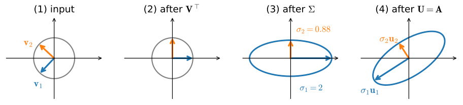
The orthonormal input direction \(\mathbf{v}_i\) is sent to the orthonormal output direction \(\mathbf{u}_i\), stretched by \(\sigma_i\). The unit circle (sphere) of right singular vectors becomes an ellipse (ellipsoid) whose semi-axes are the \(\sigma_i\mathbf{u}_i\). This is exactly the eigen-picture of Section 24.2, generalized: there one frame served as both input and output axes because the map was symmetric; here input frame \(\mathbf{V}\) and output frame \(\mathbf{U}\) are allowed to differ, which is precisely what lets the SVD handle every matrix. Figure 24.3.1 traces this for a non-symmetric \(2\times2\) matrix, so that \(\mathbf{U}\neq\mathbf{V}\) is visible: the unit circle and its right singular vectors \(\mathbf{v}_1,\mathbf{v}_2\) are rotated by \(\mathbf{V}^\top\) onto the axes, scaled by \(\boldsymbol{\Sigma}\), then rotated by \(\mathbf{U}\) so the semi-axes land along the output frame \(\sigma_1\mathbf{u}_1,\sigma_2\mathbf{u}_2\), a different orientation than the input frame, because the matrix rotates as well as stretches.
The polar decomposition: rotate–scale–rotate, rigorously. The phrase “rotate–scale–rotate” can be made precise. For square \(\mathbf{A}\), insert \(\mathbf{V}\mathbf{V}^\top=\mathbf{I}\):
\[ \mathbf{A} = \mathbf{U}\boldsymbol{\Sigma}\mathbf{V}^\top = (\mathbf{U}\mathbf{V}^\top)\,(\mathbf{V}\boldsymbol{\Sigma}\mathbf{V}^\top) = \mathbf{Q}\,\mathbf{P}. \tag{24.3.3}\]
Here \(\mathbf{Q}=\mathbf{U}\mathbf{V}^\top\) is orthogonal (a product of orthogonal matrices) and \(\mathbf{P}=\mathbf{V}\boldsymbol{\Sigma}\mathbf{V}^\top\) is symmetric positive semidefinite (its eigendecomposition has the non-negative \(\sigma_i\) as eigenvalues). This polar decomposition says every linear map is a positive-semidefinite stretch \(\mathbf{P}\) followed by a rigid rotation \(\mathbf{Q}\): the exact matrix analog of writing a complex number as \(z=re^{i\theta}\), modulus times phase. It justifies the rotate–scale–rotate slogan: the “scale” is \(\mathbf{P}\) and the net “rotate” is \(\mathbf{Q}\).
Thin SVD and the dyadic sum. If \(r=\operatorname{rank}\mathbf{A}\), only the first \(r\) singular values are nonzero. Discarding the zero columns of \(\boldsymbol{\Sigma}\) and the matching singular vectors gives the thin (or economy) SVD \(\mathbf{A}=\mathbf{U}_r\boldsymbol{\Sigma}_r\mathbf{V}_r^\top\) with \(\mathbf{U}_r\in\mathbb{R}^{m\times r}\), \(\mathbf{V}_r\in\mathbb{R}^{n\times r}\). Multiplying out, the SVD is a sum of rank-one dyads,
\[ \mathbf{A} = \sum_{i=1}^{r} \sigma_i\,\mathbf{u}_i\mathbf{v}_i^\top, \tag{24.3.4}\]
each term a single outer product weighted by its singular value, ordered from largest to smallest. This ordered list of rank-one terms is the key to the low-rank approximation of Section 24.3.2.1: retain the leading terms and discard the smaller ones.
The dyadic sum is also a one-line einsum in the Einstein notation of Section 24.1. Summing \(\sigma_i\,\mathbf{u}_i\mathbf{v}_i^\top\) over \(i\) is the index pattern 'i,mi,in->mn' (row \(i\) of Vt is \(\mathbf{v}_i^\top\)), and it rebuilds the matrix exactly:
rng = np.random.default_rng(5)
A = rng.standard_normal((4, 3))
U, s, Vt = np.linalg.svd(A, full_matrices=False)   # thin SVD
A_dyads = np.einsum('i,mi,in->mn', s, U, Vt)       # sum_i sigma_i u_i v_i^T
print('dyadic rebuild error:', round(float(np.linalg.norm(A_dyads - A)), 12))
dyadic rebuild error: 0.024.3.1.2 Existence via \(\mathbf{A}^\top\mathbf{A}\)
The SVD is the spectral theorem of Section 24.2.3.1 applied to the symmetric PSD matrix \(\mathbf{A}^\top\mathbf{A}\). A central part of the construction is that the \(\mathbf{u}_i\) are automatically orthonormal.
Proof of Equation 24.3.1 (existence). The matrix \(\mathbf{A}^\top\mathbf{A}\) is symmetric and positive semidefinite (recall Section 24.2.3.2: \(\mathbf{x}^\top(\mathbf{A}^\top\mathbf{A})\mathbf{x} = \|\mathbf{A}\mathbf{x}\|^2 \ge 0\)). By the spectral theorem it has an orthonormal eigenbasis \(\mathbf{v}_1,\ldots,\mathbf{v}_n\) with real eigenvalues, non-negative by positive semidefiniteness; order them \(\lambda_1\ge\cdots\ge\lambda_n\ge0\) and set
\[ \sigma_i = \sqrt{\lambda_i}, \qquad r = \#\{i : \sigma_i > 0\} . \]
For each \(i\le r\) define \(\mathbf{u}_i = \mathbf{A}\mathbf{v}_i/\sigma_i\). These left singular vectors are automatically orthonormal, and this single line is why:
\[ \mathbf{u}_i^\top\mathbf{u}_j = \frac{1}{\sigma_i\sigma_j}\,\mathbf{v}_i^\top\mathbf{A}^\top\mathbf{A}\,\mathbf{v}_j = \frac{1}{\sigma_i\sigma_j}\,\mathbf{v}_i^\top(\lambda_j\mathbf{v}_j) = \frac{\lambda_j}{\sigma_i\sigma_j}\,\delta_{ij} = \delta_{ij} . \]
Orthonormality of the output frame is inherited from orthonormality of the input frame, routed through \(\mathbf{A}^\top\mathbf{A}\). Extend \(\mathbf{u}_1,\ldots,\mathbf{u}_r\) to an orthonormal basis \(\mathbf{u}_1,\ldots,\mathbf{u}_m\) of \(\mathbb{R}^m\) (Gram–Schmidt on any completion). For the remaining right singular vectors, \(i>r\), we have \(\|\mathbf{A}\mathbf{v}_i\|^2=\mathbf{v}_i^\top\mathbf{A}^\top\mathbf{A}\mathbf{v}_i=\lambda_i=0\), so \(\mathbf{A}\mathbf{v}_i=\mathbf 0\). In all cases, then, \(\mathbf{A}\mathbf{v}_i=\sigma_i\mathbf{u}_i\) (with \(\sigma_i=0\) for \(i>r\)). Collecting these columns gives \(\mathbf{A}\mathbf{V}=\mathbf{U}\boldsymbol{\Sigma}\), and right-multiplying by \(\mathbf{V}^\top=\mathbf{V}^{-1}\) yields \(\mathbf{A}=\mathbf{U}\boldsymbol{\Sigma}\mathbf{V}^\top\). \(\blacksquare\)
This proof also gives a direct construction of the SVD: diagonalize the symmetric matrix \(\mathbf{A}^\top\mathbf{A}\), take square roots for the singular values, and push the eigenvectors through \(\mathbf{A}\) for the left singular vectors.
Uniqueness. The singular values are unique: they are the square roots of the eigenvalues of \(\mathbf{A}^\top\mathbf{A}\), which are determined by \(\mathbf{A}\). The singular vectors are unique only up to the same ambiguities we met for eigenvectors in Section 24.2: a sign flip on a pair \((\mathbf{u}_i,\mathbf{v}_i)\) for a simple \(\sigma_i\), and an arbitrary orthonormal rotation within the subspace belonging to a repeated singular value.
Variational characterization of \(\sigma_1\). There is a second route to the top singular value that needs no eigendecomposition and makes the meaning of \(\sigma_1\) plain. It is the Rayleigh quotient of Section 24.2.3.3 in disguise:
\[ \sigma_1 = \max_{\|\mathbf{x}\|=1}\|\mathbf{A}\mathbf{x}\| = \|\mathbf{A}\|_2 , \tag{24.3.5}\]
because \(\|\mathbf{A}\mathbf{x}\|^2=\mathbf{x}^\top\mathbf{A}^\top\mathbf{A}\mathbf{x}\) is maximized over unit \(\mathbf{x}\) by the Rayleigh proposition at \(\lambda_1=\sigma_1^2\), attained at \(\mathbf{x}=\mathbf{v}_1\). So \(\sigma_1\) is the most the matrix can stretch any unit vector: its operator (spectral) norm \(\|\mathbf{A}\|_2\). The remaining singular values come from the same problem with deflation: \(\sigma_k=\max\{\|\mathbf{A}\mathbf{x}\| : \|\mathbf{x}\|=1,\ \mathbf{x}\perp\mathbf{v}_1,\ldots,\mathbf{v}_{k-1}\}\), the Courant–Fischer min-max principle of Section 24.2.3.3 translated from Rayleigh quotients to singular values. This “maximum stretch” reading is the one that recurs in Eckart–Young, PCA, conditioning, and Lipschitz/spectral-norm arguments. The constructive proof is the better first proof (concrete, reusing results already established); the variational one explains better what \(\sigma_1\) means.
Relationship to the eigendecomposition. Substituting Equation 24.3.1 into the two Gram matrices gives, since \(\mathbf{U}\) and \(\mathbf{V}\) are orthogonal,
\[ \mathbf{A}^\top\mathbf{A} = \mathbf{V}\,\boldsymbol{\Sigma}^\top\boldsymbol{\Sigma}\,\mathbf{V}^\top, \qquad \mathbf{A}\mathbf{A}^\top = \mathbf{U}\,\boldsymbol{\Sigma}\boldsymbol{\Sigma}^\top\,\mathbf{U}^\top . \tag{24.3.6}\]
These are eigendecompositions: the right singular vectors are the eigenvectors of \(\mathbf{A}^\top\mathbf{A}\), the left singular vectors are the eigenvectors of \(\mathbf{A}\mathbf{A}^\top\), and the squared singular values \(\sigma_i^2\) are the shared eigenvalues. For a symmetric PSD matrix the SVD and the eigendecomposition coincide. In general they differ, and the warning example against conflating singular values with eigenvalues is the scaled rotation
\[ \mathbf{A} = \begin{bmatrix} 0 & -2\\ 1 & \phantom{-}0\end{bmatrix}, \qquad \mathbf{A}^\top\mathbf{A} = \begin{bmatrix} 1 & 0\\ 0 & 4\end{bmatrix}, \]
whose singular values are \(\{2,1\}\) (the square roots of \(\{4,1\}\)), while its eigenvalues are \(\pm i\sqrt2\) with modulus \(|\lambda|=\sqrt2\). The singular values are not the eigenvalue magnitudes; here even their geometric mean \(\sqrt{\sigma_1\sigma_2}=\sqrt2\) equals \(|\lambda|\), which is no accident: it is the matrix analog of the rotation-with-scaling reading from Section 24.2.1.3.3, with \(|\det\mathbf{A}|=\sigma_1\sigma_2=|\lambda_1\lambda_2|=2\). The determinant identity holds in general: for any square \(\mathbf{A}\), \(|\det\mathbf{A}|=\prod_i\sigma_i\), because orthogonal factors have determinant \(\pm1\), so the volume scaling of Section 24.1 is carried entirely by the diagonal stretch \(\boldsymbol{\Sigma}\).
The defective shear, finally decomposed. The shear of Section 24.2
\[ \mathbf{A} = \begin{bmatrix} 1 & 1\\ 0 & 1\end{bmatrix} \]
is defective: \(\lambda=1\) has algebraic multiplicity \(2\) but only a one-dimensional eigenspace, so it has no eigenbasis and hence no diagonal eigendecomposition. The SVD instead permits distinct input and output bases. Form
\[ \mathbf{A}^\top\mathbf{A} = \begin{bmatrix} 1 & 1\\ 1 & 2\end{bmatrix}, \]
a symmetric PSD matrix. Its characteristic polynomial is \(\lambda^2-3\lambda+1\), with roots \(\lambda_{1,2}=(3\pm\sqrt5)/2\). Hence the singular values are
\[ \sigma_1 = \sqrt{\tfrac{3+\sqrt5}{2}} = \frac{1+\sqrt5}{2} = \varphi \approx 1.618, \qquad \sigma_2 = \sqrt{\tfrac{3-\sqrt5}{2}} = \frac{1}{\varphi} = \varphi-1 \approx 0.618, \]
the golden ratio and its reciprocal (consistent with \(\sigma_1\sigma_2=|\det\mathbf{A}|=1\)). Both are positive, so the shear has rank \(2\) and an SVD \(\mathbf{A}=\mathbf{U}\boldsymbol{\Sigma}\mathbf{V}^\top\) with orthonormal factors. The obstruction to eigendecomposition was the requirement for one basis that serves on both sides of the map. The SVD avoids that requirement by choosing orthonormal input directions \(\mathbf v_i\) and output directions \(\mathbf u_i\) separately. The following calculation verifies the singular values against the golden ratio.
A = np.array([[1., 1.], [0., 1.]])
s = np.linalg.svd(A, compute_uv=False)
phi = (1 + np.sqrt(5)) / 2
print('singular values of the shear:', s.round(6))
print('golden ratio phi, 1/phi:    ', np.array([phi, 1 / phi]).round(6))
print('product sigma_1 * sigma_2 = |det A| =', round(float(s[0] * s[1]), 6))
singular values of the shear: [1.618034 0.618034]
golden ratio phi, 1/phi: [1.618034 0.618034]
product sigma_1 * sigma_2 = |det A| = 1.024.3.1.3 The Four Fundamental Subspaces
Because \(\mathbf{U}\) and \(\mathbf{V}\) are invertible, multiplying by them changes no dimensions, so \(\operatorname{rank}\mathbf{A}=\operatorname{rank}\boldsymbol{\Sigma}\), which is the number of nonzero diagonal entries:
\[ \operatorname{rank}\mathbf{A} = \#\{i : \sigma_i > 0\} = r . \tag{24.3.7}\]
This is the efficient characterization of rank promised in Section 24.1, where counting independent columns by elimination was the only tool on offer. The dyadic form Equation 24.3.4 makes the four fundamental subspaces equally explicit. Splitting the singular vectors at the index \(r\),
- the range (column space) of \(\mathbf{A}\) is \(\operatorname{span}\{\mathbf{u}_1,\ldots,\mathbf{u}_r\}\), since every output \(\mathbf{A}\mathbf{x}=\sum_{i\le r}\sigma_i(\mathbf{v}_i^\top\mathbf{x})\mathbf{u}_i\) is a combination of these;
- the null space of \(\mathbf{A}\) is \(\operatorname{span}\{\mathbf{v}_{r+1},\ldots,\mathbf{v}_n\}\), the input directions sent to zero;
- the row space (range of \(\mathbf{A}^\top\)) is \(\operatorname{span}\{\mathbf{v}_1,\ldots,\mathbf{v}_r\}\);
- the left null space (null space of \(\mathbf{A}^\top\)) is \(\operatorname{span}\{\mathbf{u}_{r+1},\ldots,\mathbf{u}_m\}\).
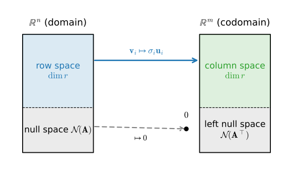
The picture is a clean bijection: \(\mathbf{A}\) maps the row space to the column space, sending each \(\mathbf{v}_i\mapsto\sigma_i\mathbf{u}_i\) (\(i\le r\)) one-to-one and onto, while mapping the null space to zero. Input space splits orthogonally as row space \(\oplus\) null space; output space splits orthogonally as column space \(\oplus\) left-null space. Figure 24.3.2 draws this two-plane map; the pseudoinverse of Section 24.3.3.1 will run the bijection backwards.
Numerical rank. In floating-point arithmetic, a matrix that is mathematically rank-deficient rarely has exact zero singular values; rounding leaves tiny \(\sigma_i\) of size around \(\epsilon_{\text{mach}}\,\sigma_1\) instead. In practice, then, rank is set by a threshold: count the singular values above a tolerance, which is exactly what np.linalg.matrix_rank does; its default cutoff is \(\sigma_1\,\max(m,n)\,\epsilon_{\text{mach}}\), scaled by both the largest singular value and the matrix size. Building a deliberately rank-2 matrix in \(\mathbb{R}^{4\times4}\) shows two singular values collapse to near machine zero, so a tolerance recovers the true rank where a test for exact zeros would fail.
rng = np.random.default_rng(0)
A = rng.standard_normal((4, 2)) @ rng.standard_normal((2, 4))  # rank <= 2
s = np.linalg.svd(A, compute_uv=False)
print('singular values:', s.round(6))
print('numerical rank :', int(np.linalg.matrix_rank(A)))
singular values: [4.351705 0.914865 0. 0. ]
numerical rank : 224.3.2 Low-Rank Approximation
24.3.2.1 Eckart–Young
The dyadic sum Equation 24.3.4 lists the rank-one pieces of \(\mathbf{A}\) in order of importance. Keeping only the top \(k\),
\[ \mathbf{A}_k = \sum_{i=1}^{k}\sigma_i\,\mathbf{u}_i\mathbf{v}_i^\top, \tag{24.3.8}\]
is the best rank-\(k\) approximation of \(\mathbf{A}\), provably, in both the spectral and Frobenius norms. Eckart and Young proved the Frobenius case (Eckart and Young 1936) and Mirsky extended it to every unitarily invariant norm (one unchanged by orthogonal multiplication on either side) (Mirsky 1960); we give the spectral-norm statement and proof in full.
Theorem (Eckart–Young–Mirsky). For every \(k<r\),
\[ \min_{\operatorname{rank}\mathbf{B}\le k}\|\mathbf{A}-\mathbf{B}\|_2 = \sigma_{k+1}, \tag{24.3.9}\]
and the minimum is attained at \(\mathbf{B}=\mathbf{A}_k\). In the Frobenius norm, \(\min_{\operatorname{rank}\mathbf{B}\le k}\|\mathbf{A}-\mathbf{B}\|_F^2=\sum_{i>k}\sigma_i^2\), again attained at \(\mathbf{A}_k\).
Proof. The truncation achieves \(\sigma_{k+1}\). The error \(\mathbf{A}-\mathbf{A}_k=\sum_{i>k}\sigma_i\mathbf{u}_i\mathbf{v}_i^\top\) is itself a (sub-)SVD whose largest singular value is \(\sigma_{k+1}\), so by the variational identity Equation 24.3.5, \(\|\mathbf{A}-\mathbf{A}_k\|_2=\sigma_{k+1}\). (And \(\|\mathbf{A}-\mathbf{A}_k\|_F^2=\sum_{i>k}\sigma_i^2\), by the identity \(\|\mathbf{A}\|_F^2=\operatorname{tr}(\mathbf{A}^\top\mathbf{A})=\sum_i\sigma_i^2\): the Frobenius norm is the root-sum-of-squares of the singular values. Exercise 2 asks you to prove this in two lines.)
No rank-\(k\) matrix does better (the dimension-counting argument). Let \(\mathbf{B}\) be any matrix with \(\operatorname{rank}\mathbf{B}\le k\). Its null space has dimension at least \(n-k\). Consider also the \((k{+}1)\)-dimensional subspace \(\mathcal{V}=\operatorname{span}\{\mathbf{v}_1,\ldots,\mathbf{v}_{k+1}\}\) spanned by the top \(k{+}1\) right singular vectors. Two subspaces of \(\mathbb{R}^n\) whose dimensions add to more than \(n\) must intersect nontrivially:
\[ \dim(\ker\mathbf{B}\cap\mathcal{V}) \ge (n-k) + (k+1) - n = 1 . \]
So there is a unit vector \(\mathbf{x}\in\ker\mathbf{B}\cap\mathcal{V}\). Write it in the top singular basis, \(\mathbf{x}=\sum_{i\le k+1}c_i\mathbf{v}_i\) with \(\sum c_i^2=1\). Because \(\mathbf{x}\in\ker\mathbf{B}\) we have \(\mathbf{B}\mathbf{x}=\mathbf 0\), and because \(\mathbf{A}\mathbf{v}_i=\sigma_i\mathbf{u}_i\) with the \(\mathbf{u}_i\) orthonormal,
\[ \|\mathbf{A}\mathbf{x}\|^2 = \Bigl\|\sum_{i\le k+1}c_i\sigma_i\mathbf{u}_i\Bigr\|^2 = \sum_{i\le k+1} c_i^2\sigma_i^2 \ge \sigma_{k+1}^2 \sum_{i\le k+1} c_i^2 = \sigma_{k+1}^2 , \]
using \(\sigma_i\ge\sigma_{k+1}\) for \(i\le k+1\). Therefore
\[ \|\mathbf{A}-\mathbf{B}\|_2^2 \ge \|(\mathbf{A}-\mathbf{B})\mathbf{x}\|^2 = \|\mathbf{A}\mathbf{x}\|^2 \ge \sigma_{k+1}^2 , \]
so \(\|\mathbf{A}-\mathbf{B}\|_2\ge\sigma_{k+1}\) for every rank-\(k\) \(\mathbf{B}\), with equality at \(\mathbf{A}_k\). \(\blacksquare\)
The kernel of \(\mathbf{B}\) and the top-\((k{+}1)\) singular subspace are subspaces of \(\mathbb{R}^n\) whose dimensions sum to more than the ambient dimension, so they must share a direction. On that direction, \(\mathbf{B}\) vanishes: \(\mathbf{B}\mathbf{x}=\mathbf 0\), while \(\mathbf{A}\) still stretches by at least \(\sigma_{k+1}\), so no rank-\(k\) \(\mathbf{B}\) can approximate \(\mathbf{A}\) more closely in every direction.
For the Frobenius norm, the case PCA relies on, the same conclusion follows from a one-line singular-value inequality, which we state as a lemma and cite rather than prove.
Lemma (Weyl’s inequality for singular values (Horn and Johnson 2012)). For matrices \(\mathbf{X},\mathbf{Y}\) of the same shape and all valid indices \(i,j\),
\[ \sigma_{i+j-1}(\mathbf{X}+\mathbf{Y})\le\sigma_i(\mathbf{X})+\sigma_j(\mathbf{Y}) . \]
Proof (Frobenius case). The lemma applied with \(\mathbf{X}=\mathbf{A}-\mathbf{B}\), \(\mathbf{Y}=\mathbf{B}\) and \(j=k{+}1\) gives \(\sigma_{k+i}(\mathbf{A})\le\sigma_i(\mathbf{A}-\mathbf{B})+\sigma_{k+1}(\mathbf{B})=\sigma_i(\mathbf{A}-\mathbf{B})\), since \(\mathbf{B}\) has rank \(\le k\) and so \(\sigma_{k+1}(\mathbf{B})=0\). Squaring and summing over \(i\ge1\),
\[ \|\mathbf{A}-\mathbf{B}\|_F^2=\sum_{i\ge1}\sigma_i(\mathbf{A}-\mathbf{B})^2 \ge\sum_{i\ge1}\sigma_{k+i}(\mathbf{A})^2=\sum_{j>k}\sigma_j(\mathbf{A})^2 , \]
again with equality at the truncation \(\mathbf{A}_k\). \(\blacksquare\)
The error formulas provide a criterion for choosing the rank. The fraction of “energy” retained by the rank-\(k\) truncation is the energy ratio
\[ \frac{\sum_{i\le k}\sigma_i^2}{\sum_{i}\sigma_i^2} = 1 - \frac{\|\mathbf{A}-\mathbf{A}_k\|_F^2}{\|\mathbf{A}\|_F^2} , \tag{24.3.10}\]
so choosing \(k\) to capture, say, 95% of the energy is a principled way to set the rank. When the singular values decay quickly (as they do for images with large-scale structure and, empirically, for many trained weight matrices), a small \(k\) captures most of the Frobenius norm, and low-rank compression is then effective.
Truncation as denoising. There is a second, statistical reason to truncate. Suppose the observed matrix is a low-rank signal plus noise, \(\mathbf{A}=\mathbf{B}+\mathbf{N}\), where \(\mathbf{A}\in\mathbb R^{m\times n}\), \(\operatorname{rank}\mathbf{B}=r\), and the entries of \(\mathbf N\) are independent, mean zero, and have standard deviation \(\sigma_{\text{noise}}\). In the large-dimensional iid model, the noise singular values lie below an edge near \((\sqrt{m}+\sqrt{n})\sigma_{\text{noise}}\). A sufficiently strong signal can produce singular values beyond this edge; weak components need not separate from the noise bulk. Truncation above an appropriate threshold can therefore reduce error, but the location of that threshold depends on the model.
Under the square-matrix model with known noise level, Gavish and Donoho derive the asymptotically optimal hard threshold \(\tfrac{4}{\sqrt3}\sqrt n\,\sigma_{\mathrm{noise}}\approx2.309\sqrt n\,\sigma_{\mathrm{noise}}\) (Gavish and Donoho 2014). Applying this constant to a different aspect ratio, noise distribution, normalization, or unknown-noise setting requires the corresponding version of the theory. Exercise 3 illustrates the spectral separation; it does not establish the asymptotic result.
The same low-rank premise, with missing rather than noisy entries, is matrix completion: recommender systems fill in a sparsely observed ratings matrix by seeking the lowest-rank matrix consistent with the observed entries, in practice by minimizing the nuclear norm \(\|\mathbf{A}\|_*=\sum_i\sigma_i\), the convex stand-in for rank (Candès and Recht 2009). The nuclear norm plays the role for rank that the \(\ell_1\) norm plays for sparsity.
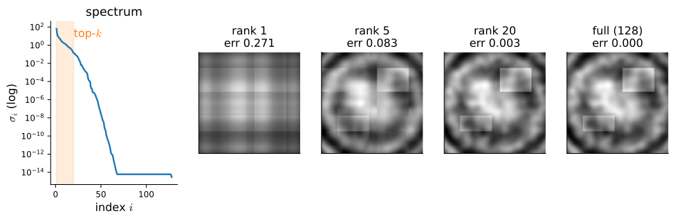
Figure 24.3.3 makes this concrete on a grayscale image. The left panel plots the singular-value spectrum on a log scale (note the rapid decay); the remaining panels reconstruct the image at ranks \(k=1,5,20\) and full, each labeled with its relative Frobenius error
\[ \|\mathbf{A}-\mathbf{A}_k\|_F/\|\mathbf{A}\|_F=\sqrt{\sum_{i>k}\sigma_i^2/\sum_i\sigma_i^2}. \]
For this image, the rank-20 truncation has small relative Frobenius error and retains the visually dominant structure. The panels illustrate the approximation theorem; the algebraic argument above supplies its proof.
24.3.2.2 Principal Component Analysis
Principal component analysis is a direct application of the SVD and the Eckart–Young theorem. Given data points as the rows of \(\mathbf{X}\in\mathbb{R}^{n\times d}\), first center them by subtracting the mean row, \(\tilde{\mathbf{X}}=\mathbf{X}-\mathbf 1\bar{\mathbf{x}}^\top\). The empirical covariance is the symmetric PSD matrix \(\mathbf{C}=\tfrac1n\tilde{\mathbf{X}}^\top\tilde{\mathbf{X}}\) from Section 24.2.3.2 (we use the maximum-likelihood \(\tfrac1n\) covariance; the unbiased \(\tfrac1{n-1}\) version rescales every eigenvalue by the same factor and so changes neither the principal directions nor the explained-variance ratio). PCA asks: which unit direction \(\mathbf{w}\) captures the most variance of the projected data?
Proposition (PCA via Rayleigh). The projected variance \(\tfrac1n\|\tilde{\mathbf{X}}\mathbf{w}\|^2=\mathbf{w}^\top\mathbf{C}\mathbf{w}\) is maximized over unit \(\mathbf{w}\) by the top eigenvector of \(\mathbf{C}\), which is the top right singular vector \(\mathbf{v}_1\) of \(\tilde{\mathbf{X}}\), with maximal variance \(\sigma_1^2/n\).
Proof. The projection of a centered point onto \(\mathbf{w}\) has coordinate \(\tilde{\mathbf{x}}^\top\mathbf{w}\); the variance of these coordinates is \(\tfrac1n\sum_i(\tilde{\mathbf{x}}_i^\top\mathbf{w})^2=\tfrac1n\|\tilde{\mathbf{X}}\mathbf{w}\|^2=\mathbf{w}^\top\mathbf{C}\mathbf{w}\). Maximizing this Rayleigh quotient over unit \(\mathbf{w}\) gives, by Section 24.2.3.3, the top eigenvector of \(\mathbf{C}\) and the value \(\lambda_1(\mathbf{C})\). By Equation 24.3.6, \(\mathbf{C}=\tfrac1n\mathbf{V}\boldsymbol{\Sigma}^\top\boldsymbol{\Sigma}\mathbf{V}^\top\), so its eigenvectors are the right singular vectors \(\mathbf{v}_i\) of \(\tilde{\mathbf{X}}\) and its eigenvalues are \(\sigma_i^2/n\). \(\blacksquare\)
Iterating with deflation, the top-\(k\) principal directions are \(\mathbf{v}_1,\ldots,\mathbf{v}_k\), and the variance explained by component \(i\) is \(\sigma_i^2/n\). The ranked list of these variances is the scree plot, and the explained-variance ratio is exactly the energy ratio Equation 24.3.10 of \(\tilde{\mathbf{X}}\). Moreover the rank-\(k\) projection \(\mathbf{z}=\mathbf{V}_k^\top(\mathbf{x}-\bar{\mathbf{x}})\) is the optimal linear dimensionality reduction: minimizing reconstruction error over all rank-\(k\) linear maps is Eckart–Young–Frobenius applied to \(\tilde{\mathbf{X}}\), whose solution is the top-\(k\) truncation. Centering matters: skip it and the first singular vector is dominated by the offset of the cloud from the origin, capturing where the data is rather than how it varies.
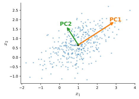
Figure 24.3.4 draws a 2-D correlated cloud with its two principal axes scaled by the per-axis standard deviation \(\sigma_i/\sqrt{n}\): the first axis aligns with the long direction of the cloud, exactly the direction of maximal variance the proposition predicts. The cell below cross-checks the SVD principal axes against the eigenvectors of the covariance and reports the explained-variance ratio; the two routes agree, as Equation 24.3.6 guarantees.
rng = np.random.default_rng(1)
theta = np.pi / 5
rot = np.array([[np.cos(theta), -np.sin(theta)],
                [np.sin(theta),  np.cos(theta)]])
X = rng.standard_normal((300, 2)) * np.array([3.0, 0.8]) @ rot.T  # correlated
Xc = X - X.mean(0)                                                # center
s = np.linalg.svd(Xc, compute_uv=False)
eigval = np.linalg.eigvalsh((Xc.T @ Xc) / len(Xc))[::-1]          # descending
print('explained variance (sigma^2/n):', (s ** 2 / len(Xc)).round(4))
print('eigenvalues of covariance     :', eigval.round(4))
print('explained-variance ratio      :', (s ** 2 / (s ** 2).sum()).round(4))
explained variance (sigma^2/n): [8.0873 0.5705]
eigenvalues of covariance : [8.0873 0.5705]
explained-variance ratio : [0.9341 0.0659]24.3.3 Solving Linear Systems with the SVD
24.3.3.1 The Pseudoinverse and Least Squares
When \(\mathbf{A}\mathbf{x}=\mathbf{b}\) has no solution (too many equations) or infinitely many (too few), the right formulation is the least-squares problem Equation 24.1.9 of Section 24.1, and the SVD solves it in full generality. Define the Moore–Penrose pseudoinverse by inverting the nonzero singular values and transposing the rotations,
\[ \mathbf{A}^{+} = \mathbf{V}\boldsymbol{\Sigma}^{+}\mathbf{U}^\top, \qquad \boldsymbol{\Sigma}^{+}_{ii} = \begin{cases} 1/\sigma_i & \sigma_i>0,\\ 0 & \sigma_i=0.\end{cases} \tag{24.3.11}\]
Proposition (min-norm least squares). Among all minimizers of \(\|\mathbf{A}\mathbf{x}-\mathbf{b}\|_2\), the one of smallest norm is \(\hat{\mathbf{x}}=\mathbf{A}^{+}\mathbf{b}\).
Proof. Rotate both the input and the target into the singular bases: \(\mathbf{y}=\mathbf{V}^\top\mathbf{x}\) and \(\mathbf{c}=\mathbf{U}^\top\mathbf{b}\). Since \(\mathbf{U}\) is orthogonal it preserves norms, so
\[ \|\mathbf{A}\mathbf{x}-\mathbf{b}\|^2 = \|\mathbf{U}^\top(\mathbf{A}\mathbf{x}-\mathbf{b})\|^2 = \|\boldsymbol{\Sigma}\mathbf{y}-\mathbf{c}\|^2 = \sum_{i\le r}(\sigma_i y_i - c_i)^2 + \sum_{i> r} c_i^2 . \]
The rotation has decoupled the problem into independent scalar problems. The first sum is minimized term by term at \(y_i=c_i/\sigma_i\) for \(i\le r\); the second sum is a constant we cannot touch (it is the irreducible residual, the part of \(\mathbf{b}\) outside the column space). The coordinates \(y_i\) for \(i>r\) are free: they do not appear in the residual at all. Setting them to zero gives the unique solution of smallest norm (since \(\|\mathbf{x}\|=\|\mathbf{y}\|\)). That choice is exactly \(\mathbf{y}=\boldsymbol{\Sigma}^{+}\mathbf{c}\), i.e. \(\hat{\mathbf{x}}=\mathbf{V}\boldsymbol{\Sigma}^{+}\mathbf{U}^\top\mathbf{b}=\mathbf{A}^{+}\mathbf{b}\). \(\blacksquare\)
Rotating into the SVD basis turns a coupled least-squares problem into a list of one-dimensional problems, and “small residual” and “small norm” occupy disjoint coordinate blocks (\(i\le r\) versus \(i>r\)), so both can be satisfied at once. Two corollaries follow. When \(\mathbf{A}\) is square and invertible, all \(\sigma_i>0\) and \(\mathbf{A}^{+}=\mathbf{V}\boldsymbol{\Sigma}^{-1}\mathbf{U}^\top=\mathbf{A}^{-1}\). And truncating the pseudoinverse (dropping terms with tiny \(\sigma_i\) instead of dividing by them) caps the large \(1/\sigma_i\) factor; this is a form of regularization, closely related to ridge regression, which we revisit when we discuss weight decay in Section 2.7.
The classical alternative, the normal equations \(\mathbf{A}^\top\mathbf{A}\mathbf{x}=\mathbf{A}^\top\mathbf{b}\), is mathematically equivalent for full-rank \(\mathbf{A}\) but numerically worse: forming \(\mathbf{A}^\top\mathbf{A}\) squares the condition number (Section 24.3.3.2), so an SVD- or QR-based solve is preferred. The cell below solves an overdetermined system via pinv and via the library lstsq (the two agree on the same minimum-residual fit) and prints cond(A) alongside cond(A^T A) to show the normal-equations matrix is far worse conditioned.
A = np.array([[1., 1.], [1., 2.], [1., 3.], [1., 4.]])  # 4 eqns, 2 unknowns
b = np.array([6., 5., 7., 10.])
x_pinv = np.linalg.pinv(A) @ b
x_lstsq, *_ = np.linalg.lstsq(A, b, rcond=None)
print('pinv :', x_pinv.round(4), ' residual',
      round(float(np.linalg.norm(A @ x_pinv - b)), 4))
print('lstsq:', x_lstsq.round(4), ' residual',
      round(float(np.linalg.norm(A @ x_lstsq - b)), 4))
print('cond(A)     =', round(float(np.linalg.cond(A)), 3))
print('cond(A^T A) =', round(float(np.linalg.cond(A.T @ A)), 3), '= cond(A)^2')
pinv : [3.5 1.4] residual 2.0494
lstsq: [3.5 1.4] residual 2.0494
cond(A) = 7.469
cond(A^T A) = 55.782 = cond(A)^224.3.3.2 The Condition Number
The condition number is the single SVD-derived scalar that predicts numerical error amplification. For an invertible (or full-rank) matrix it is the ratio of the largest to the smallest nonzero singular value,
\[ \kappa(\mathbf{A}) = \frac{\sigma_1}{\sigma_r} . \tag{24.3.12}\]
It measures how much a linear solve can amplify input error.
Proposition (error amplification, with tightness). Let \(\mathbf{A}\) be square invertible, \(\mathbf{A}\mathbf{x}=\mathbf{b}\), and let a perturbation \(\delta\mathbf{b}\) change the solution to \(\mathbf{x}+\delta\mathbf{x}\). Then
\[ \frac{\|\delta\mathbf{x}\|}{\|\mathbf{x}\|} \le \kappa(\mathbf{A})\,\frac{\|\delta\mathbf{b}\|}{\|\mathbf{b}\|}, \tag{24.3.13}\]
and the bound is attained for suitable \(\mathbf{b},\delta\mathbf{b}\).
Proof. From \(\mathbf{A}\,\delta\mathbf{x}=\delta\mathbf{b}\) we get \(\delta\mathbf{x}=\mathbf{A}^{-1}\delta\mathbf{b}\), and the largest singular value of \(\mathbf{A}^{-1}\) is \(1/\sigma_n\), so by Equation 24.3.5 \(\|\delta\mathbf{x}\|\le\sigma_n^{-1}\|\delta\mathbf{b}\|\). From \(\mathbf{b}=\mathbf{A}\mathbf{x}\) we get \(\|\mathbf{b}\|\le\sigma_1\|\mathbf{x}\|\). Multiplying the two inequalities,
\[ \frac{\|\delta\mathbf{x}\|}{\|\mathbf{x}\|} \le \frac{\sigma_1}{\sigma_n}\,\frac{\|\delta\mathbf{b}\|}{\|\mathbf{b}\|} = \kappa(\mathbf{A})\,\frac{\|\delta\mathbf{b}\|}{\|\mathbf{b}\|} . \]
It is tight: align the signal with the direction the inverse amplifies least by taking \(\mathbf{b}=\mathbf{u}_1\), so that \(\mathbf{x}=\sigma_1^{-1}\mathbf{v}_1\) is the smallest-norm solution any unit right-hand side can produce (a small \(\|\mathbf{x}\|\) in the denominator is exactly what maximizes the relative-error ratio), and align the error with the most-amplified direction \(\delta\mathbf{b}=\mathbf{u}_n\) (so \(\delta\mathbf{x}=\sigma_n^{-1}\mathbf{v}_n\) is as large as a perturbation of its size can get); then both inequalities are equalities. \(\blacksquare\)
Three consequences follow. An orthogonal matrix has all singular values equal to \(1\), so \(\kappa=1\): rotations and reflections are perfectly conditioned, which is why the SVD’s \(\mathbf{U},\mathbf{V}\) never amplify error and why orthogonal initialization is attractive. At the other extreme, forming the normal-equations matrix squares the conditioning, \(\kappa(\mathbf{A}^\top\mathbf{A})=\kappa(\mathbf{A})^2\) (its singular values are the \(\sigma_i^2\)), which is the quantitative reason to prefer an SVD/QR least-squares solve over the normal equations (Section 24.3.3.1).
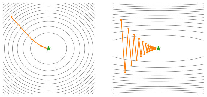
Geometrically, a large \(\kappa\) means very elongated level sets. For a quadratic bowl \(f(\mathbf{x})=\tfrac12\mathbf{x}^\top\mathbf{M}\mathbf{x}\) with \(\mathbf{M}\) symmetric positive definite, the contours are ellipses whose axis ratio is exactly \(\sqrt{\kappa(\mathbf{M})}=\sqrt{\lambda_{\max}/\lambda_{\min}}\); when \(\kappa\gg1\) the bowl is a narrow valley, and gradient descent zig-zags across the steep walls while crawling along the flat floor. (For a least-squares objective \(\tfrac12\|\mathbf{A}\mathbf{x}-\mathbf{b}\|^2\) the bowl’s matrix is \(\mathbf{M}=\mathbf{A}^\top\mathbf{A}\), so its geometric axis ratio is \(\kappa(\mathbf A)\) while the Hessian condition number that controls gradient descent is \(\kappa(\mathbf A)^2\).) This is the same picture that ended the Rayleigh discussion in Section 24.2.3.3, and it is no coincidence: with the best fixed step size, gradient descent’s error contracts like \((\kappa-1)/(\kappa+1)\) per step on such a bowl. One number, two consequences: error amplification in a solve and slow convergence in optimization. We make this precise when we analyze gradient descent in Section 26.1 and study numerical conditioning in Section 26.5. Figure 24.3.5 contrasts a well-conditioned bowl (\(\kappa\approx1\), near-circular contours, gradient descent heads almost straight to the minimum) with an ill-conditioned one (\(\kappa\gg1\), elongated contours, a zig-zag trajectory). In the narrow valley, the step size is throttled by the steep direction (to stay stable) while the flat direction needs many such small steps to make progress; the zig-zag is the visible cost of a large condition number.
24.3.4 The SVD in Modern Deep Learning
Low-rank structure is everywhere in contemporary models, and Eckart–Young is the reason it can be exploited cheaply.
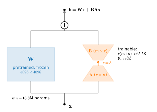
Low-rank adapters (LoRA). Fine-tuning a large pretrained model by updating every weight is expensive. LoRA (Hu et al. 2021) freezes a pretrained weight \(\mathbf{W}\in\mathbb{R}^{m\times n}\) and learns only a low-rank correction \(\Delta\mathbf{W}=\mathbf{B}\mathbf{A}\) with \(\mathbf{B}\in\mathbb{R}^{m\times r}\), \(\mathbf{A}\in\mathbb{R}^{r\times n}\), and \(r\ll\min(m,n)\). This trades \(mn\) trainable parameters for \(r(m+n)\), a ratio of
\[ \frac{r(m+n)}{mn} , \tag{24.3.14}\]
which for a \(4096\times4096\) layer at rank \(r=8\) is \(8\cdot8192/4096^2\approx0.39\%\) of the parameters. Figure 24.3.6 shows the architecture: the frozen weight and the trainable low-rank bypass act on the same input, and their outputs add. The hypothesis that fine-tuning updates are intrinsically low rank is what makes this work.
Note what Eckart–Young does and does not say here: LoRA learns \(\mathbf{B}\) and \(\mathbf{A}\) by gradient descent rather than truncating a known matrix, so the theorem promises nothing about the learned adapter itself. What it quantifies is the ceiling: if the update that full fine-tuning would have made has singular values \(\sigma_1\ge\sigma_2\ge\cdots\), then no rank-\(r\) adapter can approximate it with error below \(\sigma_{r+1}\) in spectral norm (\(\sum_{i>r}\sigma_i^2\) in squared Frobenius norm), so the approach can only succeed when the true update’s spectrum decays fast, which is exactly the empirical finding that motivated LoRA. PiSSA makes the link to the SVD literal: it initializes \(\mathbf{B}\) and \(\mathbf{A}\) from the truncated SVD of the pretrained weight \(\mathbf{W}\) itself, so that fine-tuning starts by adapting the principal components (Meng et al. 2024).
Orthogonalized updates (Muon). The polar decomposition Equation 24.3.3 underlies Muon (Jordan et al. 2024), an optimizer adopted in recent large-scale language-model training. Write the momentum matrix of a weight as \(\mathbf{M}=\mathbf{U}\boldsymbol{\Sigma}\mathbf{V}^\top\); the momentum is the running average of gradients that optimizers keep per weight (see the optimization chapters). A standard momentum step moves along \(\mathbf{M}\), which is dominated by its few largest dyads; Muon instead steps along the polar factor \(\mathbf{Q}=\mathbf{U}\mathbf{V}^\top\), the rotation part of the update with every stretch factor equalized to \(1\), so rare-but-consistent gradient directions are not drowned out by the dominant ones. (Equivalently, \(\mathbf{U}\mathbf{V}^\top\) is the steepest-descent direction when distances between weight matrices are measured in the spectral norm rather than the Euclidean one (Bernstein and Newhouse 2024).) Computing an SVD of every weight at every step would be hopeless; instead Muon runs a handful of Newton–Schulz iterations \(\mathbf{X}\leftarrow\tfrac12(3\mathbf{X}-\mathbf{X}\mathbf{X}^\top\mathbf{X})\) starting from \(\mathbf{X}=\mathbf{M}/\|\mathbf{M}\|_F\). Each iteration leaves \(\mathbf{U}\) and \(\mathbf{V}\) untouched and applies the odd polynomial \(p(\sigma)=\tfrac12(3\sigma-\sigma^3)\) to every singular value, driving each nonzero \(\sigma_i\) toward the fixed point \(1\). The Frobenius normalization is what makes that convergence guaranteed rather than lucky: it puts every singular value into \((0, 1]\), comfortably inside \((0, \sqrt3\,)\), the cubic’s basin of attraction of \(1\). Start a singular value beyond \(\sqrt3\) and the cubic maps it negative, after which the iterates either stick near the spurious fixed point \(-1\) or diverge; either way the polar factor is lost. So the iterates converge to \(\mathbf{U}\mathbf{V}^\top\) using nothing but matrix multiplications (in practice Muon tunes the polynomial’s coefficients so that about five iterations suffice). Like the power iteration used for spectral normalization below, this procedure requires only matrix multiplications and is efficient on GPUs.
The following calculation illustrates the iteration. After Frobenius normalization, repeated application of the cubic maps every nonzero singular value toward \(1\) while preserving the singular vectors. The iterate therefore approaches the polar factor \(\mathbf{U}\mathbf{V}^\top\) computed by a direct SVD. With the plain \(\tfrac12(3\sigma-\sigma^3)\) coefficients, the smallest singular value (which starts closest to \(0\), where \(p\) only multiplies it by \(\tfrac32\)) converges slowest, needing about ten iterations here; Muon’s tuned polynomials accelerate exactly that small-\(\sigma\) regime.
rng = np.random.default_rng(3)
M = rng.standard_normal((6, 4))          # a stand-in momentum matrix
X = M / np.linalg.norm(M)                # Frobenius normalize: all sigma <= 1
for k in range(1, 11):
    X = 1.5 * X - 0.5 * X @ X.T @ X      # applies p(sigma) = (3 sigma - sigma^3)/2
    if k % 2 == 0:
        print(f'iter {k:2d}: sigma =', np.linalg.svd(X, compute_uv=False).round(4))
U, s, Vt = np.linalg.svd(M, full_matrices=False)
print('distance to polar factor U V^T:',
      round(float(np.linalg.norm(X - U @ Vt)), 6))
iter 2: sigma = [0.9982 0.8554 0.4648 0.1499]
iter 4: sigma = [1. 0.9987 0.8351 0.3291]
iter 6: sigma = [1. 1. 0.9978 0.6599]
iter 8: sigma = [1. 1. 1. 0.9663]
iter 10: sigma = [1. 1. 1. 1.]
distance to polar factor U V^T: 4e-06Spectral normalization. Constraining the largest singular value of each weight matrix to \(1\) caps the per-layer Lipschitz constant, the largest factor by which the layer can stretch any input difference (Equation 24.3.5: \(\sigma_1=\|\mathbf{W}\|_2\)). This stabilizes training, originally for GAN discriminators (Miyato et al. 2018). \(\sigma_1\) is estimated by power iteration on \(\mathbf{W}^\top\mathbf{W}\), the very algorithm we analyzed in Section 24.2, since \(\sigma_1=\sqrt{\lambda_1(\mathbf{W}^\top\mathbf{W})}\). A couple of iterations per training step suffice.
Weight and attention spectra. Plotting the singular values of a trained layer (the spectrum panel of Figure 24.3.3, applied to \(\mathbf{W}\) instead of an image) reveals its effective rank via the energy ratio Equation 24.3.10 and exposes heavy-tailed spectra that correlate with generalization (Martin and Mahoney 2021), heavy-tailed precisely against the Marchenko–Pastur noise baseline of Section 24.2.
Attention matrices are often empirically near-low-rank, which motivates linear-attention approximations that replace the full softmax attention with a low-rank surrogate. The most prominent recent instance is low-rank key–value compression: DeepSeek-V2’s multi-head latent attention stores a single low-rank latent in place of the full per-head key–value cache (the cached per-token keys and values that dominate inference memory) and expands it on the fly (DeepSeek-AI 2024).
The cell below makes the weight-side diagnostic concrete: it builds a synthetic weight matrix with a fast-decaying spectrum and reports the rank needed for 95% spectral energy and the parameter saving a LoRA of that rank would give; here rank 18 of 256, about 10.5% of the full parameter count. How small that rank is depends entirely on how fast the spectrum decays (compare the 0.39% headline above, which assumed \(r=8\) suffices), which is why one measures the spectrum instead of assuming a rank.
rng = np.random.default_rng(2)
m, n = 256, 512
sigma = np.exp(-np.arange(min(m, n)) / 12.0)                 # fast-decaying spectrum
Uw, _ = np.linalg.qr(rng.standard_normal((m, min(m, n))))
Vw, _ = np.linalg.qr(rng.standard_normal((n, min(m, n))))
s = np.linalg.svd((Uw * sigma) @ Vw.T, compute_uv=False)
r95 = int(np.searchsorted(np.cumsum(s ** 2) / (s ** 2).sum(), 0.95) + 1)
print(f'{m} x {n} matrix; rank for 95% energy: {r95}; '
      f'LoRA params {r95 * (m + n) / (m * n):.1%} of full')
256 x 512 matrix; rank for 95% energy: 18; LoRA params 10.5% of fullScaling up. For matrices too large to factor fully, randomized SVD (Halko et al. 2011) computes an accurate rank-\(k\) truncation at a fraction of the cost. The mechanism is a range finder: draw a random \(n\times(k{+}p)\) Gaussian matrix \(\boldsymbol\Omega\) (a small oversampling \(p\) guards against unlucky draws), form \(\mathbf{Y}=\mathbf{A}\boldsymbol\Omega\) (a handful of matrix–vector products that sketch the column space), and orthonormalize it, \(\mathbf{Q}=\operatorname{qr}(\mathbf{Y})\). Because \(\mathbf{A}\)’s energy is concentrated in its top singular directions, the \(k{+}p\) columns of \(\mathbf{Q}\) capture them with high probability, so one then factors only the tiny matrix \(\mathbf{Q}^\top\mathbf{A}\) and maps its left singular vectors back through \(\mathbf{Q}\). The cost drops from the \(O(mn\min(m,n))\) of a full SVD to a few passes over \(\mathbf{A}\); this method is useful when only the leading singular triples are needed. A related family, CUR decompositions, approximates \(\mathbf{A}\) with actual rows and columns of \(\mathbf{A}\), trading accuracy for interpretability.
We finish with a numerical check that the SVD reconstructs \(\mathbf{A}\) and that \(\sigma_i^2\) are the eigenvalues of \(\mathbf{A}^\top\mathbf{A}\).
A = np.array([[3., 1.], [1., 3.], [0., 2.]])   # a 3x2 matrix
U, s, Vt = np.linalg.svd(A, full_matrices=False)
recon = (U * s) @ Vt
eig = np.sort(np.linalg.eigvalsh(A.T @ A))[::-1]
print('reconstruction error:', round(float(np.linalg.norm(recon - A)), 12))
print('sigma^2          :', (s ** 2).round(6))
print('eig(A^T A) sorted:', eig.round(6))
reconstruction error: 0.0
sigma^2 : [18.324555 5.675445]
eig(A^T A) sorted: [18.324555 5.675445]The reconstruction error is at the level of floating-point round-off, and the squared singular values match the eigenvalues of \(\mathbf{A}^\top\mathbf{A}\): exactly the construction of Section 24.3.1.2.
24.3.5 Summary
- Every matrix factors as \(\mathbf{A}=\mathbf{U}\boldsymbol{\Sigma}\mathbf{V}^\top\) (rotate–scale–rotate; equivalently the polar form \(\mathbf{A}=\mathbf{Q}\mathbf{P}\)), with \(\mathbf{A}\mathbf{v}_i=\sigma_i\mathbf{u}_i\) and the dyadic sum \(\mathbf{A}=\sum_i\sigma_i\mathbf{u}_i\mathbf{v}_i^\top\).
- The SVD is the spectral theorem applied to the symmetric PSD matrix \(\mathbf{A}^\top\mathbf{A}\), with \(\sigma_i=\sqrt{\lambda_i(\mathbf{A}^\top\mathbf{A})}\); it therefore exists even for the defective shear that had no eigenbasis. Equivalently \(\sigma_1=\max_{\|\mathbf{x}\|=1}\|\mathbf{A}\mathbf{x}\|=\|\mathbf{A}\|_2\).
- Rank, range, and the four fundamental subspaces read off the spectrum; numerical rank thresholds the \(\sigma_i\) at \(\sim\sigma_1\max(m,n)\,\epsilon_{\text{mach}}\).
- Eckart–Young–Mirsky: the top-\(k\) truncation \(\mathbf{A}_k\) is the optimal rank-\(k\) approximation, with \(\|\mathbf{A}-\mathbf{A}_k\|_2=\sigma_{k+1}\) and \(\|\mathbf{A}-\mathbf{A}_k\|_F^2=\sum_{i>k}\sigma_i^2\). The retained-energy ratio \(\sum_{i\leq k}\sigma_i^2/\sum_i\sigma_i^2\) is one minus the squared relative Frobenius error.
- PCA is Eckart–Young on centered data: principal directions are the right singular vectors \(\mathbf{v}_i\), explained variance is \(\sigma_i^2/n\).
- The pseudoinverse \(\mathbf{A}^{+}=\mathbf{V}\boldsymbol{\Sigma}^{+}\mathbf{U}^\top\) gives the minimum-norm least-squares solution; the condition number \(\kappa=\sigma_1/\sigma_r\) predicts both error amplification and gradient-descent speed, and \(\kappa(\mathbf{A}^\top\mathbf{A})=\kappa(\mathbf{A})^2\) is why the normal equations are worse.
- SVD powers PCA, LoRA (rank-\(r\) updates at \(r(m+n)\) parameters), Muon (steps along the polar factor \(\mathbf{U}\mathbf{V}^\top\), computed by Newton–Schulz iterations), spectral normalization (power iteration on \(\mathbf{W}^\top\mathbf{W}\)), and weight / attention spectral analysis.
24.3.6 Exercises
- Compute the SVD of \(\operatorname{diag}(3,1)\) by inspection. Then show the scaled rotation \(\begin{bmatrix}0&-2\\1&0\end{bmatrix}\) has singular values \(\{2,1\}\) even though its eigenvalue magnitudes are both \(\sqrt2\), i.e. \(\sigma\neq|\lambda|\) for non-symmetric matrices.
- Prove that \(\|\mathbf{A}\|_F^2=\sum_i\sigma_i^2\). (Hint: first show \(\|\mathbf{A}\|_F^2=\operatorname{tr}(\mathbf{A}^\top\mathbf{A})\) directly from the definitions, then evaluate the trace as the sum of the eigenvalues of \(\mathbf{A}^\top\mathbf{A}\) using Equation 24.3.6.) Conclude that multiplying by orthogonal matrices on either side never changes the Frobenius norm.
- Generate a rank-5 signal \(\mathbf{B}=\mathbf{X}\mathbf{Y}^\top\) with \(\mathbf{X},\mathbf{Y}\in\mathbb{R}^{200\times5}\) standard Gaussian, and add noise \(\mathbf{N}\) with i.i.d. \(\mathcal{N}(0,\sigma_{\text{noise}}^2)\) entries, \(\sigma_{\text{noise}}=0.05\). Plot the singular values of \(\mathbf{B}+\mathbf{N}\) on a log scale and examine the separation between five signal values and a noise floor near \((\sqrt{m}+\sqrt{n})\,\sigma_{\text{noise}}\). Verify that hard-thresholding at the Gavish–Donoho cutoff \(\tfrac{4}{\sqrt3}\sqrt{n}\,\sigma_{\text{noise}}\) recovers the true rank, and check numerically whether the rank-5 truncation of \(\mathbf{B}+\mathbf{N}\) is closer to \(\mathbf{B}\) (in Frobenius norm) than \(\mathbf{B}+\mathbf{N}\) itself is. What happens as you keep more components than 5?
- Show that the singular values of any orthogonal matrix are all \(1\), hence \(\kappa=1\). Then prove \(\kappa(\mathbf{A}^\top\mathbf{A})=\kappa(\mathbf{A})^2\) and explain why this makes the normal equations numerically inferior.
- Show \(\mathbf{A}\) and \(\mathbf{A}^\top\) have the same nonzero singular values. (Hint: relate \(\mathbf{A}^\top\mathbf{A}\) and \(\mathbf{A}\mathbf{A}^\top\) via Equation 24.3.6.)
- Prove the polar decomposition \(\mathbf{A}=\mathbf{Q}\mathbf{P}\) has \(\mathbf{Q}\) orthogonal and \(\mathbf{P}\succeq0\), and that \(\mathbf{P}\) is unique while \(\mathbf{Q}\) is unique when \(\mathbf{A}\) is invertible.
- For a given weight matrix, find the LoRA rank achieving 95% spectral energy and compute the resulting parameter saving relative to a full update (the
#svd-weight-spectrumcell). How does the answer change if the spectrum decays more slowly? - How much can an update \(\boldsymbol{\Delta}\) (for instance a rank-\(r\) LoRA update \(\mathbf{B}\mathbf{A}\)) move the singular values of \(\mathbf{W}\)?
- Derive the Weyl perturbation bound \(|\sigma_i(\mathbf{W}+\boldsymbol{\Delta})-\sigma_i(\mathbf{W})|\le\sigma_1(\boldsymbol{\Delta})\) for every \(i\) and any update \(\boldsymbol{\Delta}\), by setting \(j=1\) in the Weyl inequality lemma of Section 24.3.2.1, \(\sigma_{i+j-1}(\mathbf{X}+\mathbf{Y})\le\sigma_i(\mathbf{X})+\sigma_j(\mathbf{Y})\), applied in both directions.
- Can a rank-one update move all the singular values? Take \(\mathbf{W}=\operatorname{diag}(1,2)\) and \(\boldsymbol{\Delta}=0.1\,\mathbf{1}\mathbf{1}^\top\), compute the singular values of \(\mathbf{W}+\boldsymbol{\Delta}\) numerically, and check that both moved, each by less than \(\sigma_1(\boldsymbol{\Delta})=0.2\), as the bound demands.
- Reconcile this with the fact that adding a rank-\(r\) update changes \(\operatorname{rank}\mathbf{W}\) by at most \(r\): a low-rank update can nudge every singular value a little, but can create or destroy at most \(r\) nonzero ones.