from d2l import torch as d2l
import torch
from torch import nn4.2 Implementation of Multilayer Perceptrons
An MLP implementation extends a linear classifier by composing affine layers with nonlinear activations. We first write this composition explicitly and then use the corresponding framework layers.
from d2l import tensorflow as d2l
import tensorflow as tf
from d2l import jax as d2l
from flax import nnx
from jax import numpy as jnpfrom d2l import mxnet as d2l
from mxnet import np, npx
from mxnet.gluon import nn
npx.set_np()4.2.1 Implementation from Scratch
We begin with an implementation using tensors and automatic differentiation.
4.2.1.1 Initializing Model Parameters
Recall that Fashion-MNIST contains 10 classes, and that each image consists of a \(28 \times 28 = 784\) grid of grayscale pixel values. As before we will disregard the spatial structure among the pixels for now, so we can think of this as a classification dataset with 784 input features and 10 classes. To begin, we will implement an MLP with one hidden layer and 256 hidden units (Figure 4.2.1). Both the number of layers and their width are adjustable (they are considered hyperparameters). Powers-of-two widths often align well with accelerator kernels, although the fastest dimensions depend on the hardware and numerical precision.
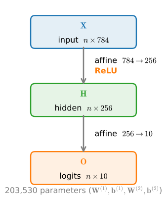
Again, we will represent our parameters with several tensors. Note that for every layer, we must keep track of one weight matrix and one bias vector. As always, we allocate memory for the gradients of the loss with respect to these parameters. We use small Gaussian noise (\(\sigma = 0.01\)) as a simple starting point; principled strategies for choosing this scale are the subject of Section 4.4.
In the code below we use nn.Parameter to automatically register a class attribute as a parameter to be tracked by autograd (Section 1.5).
In the code below we use tf.Variable to define the model parameter.
In the code below, nnx.Param marks each array as a trainable parameter.
In the code below, we first define and initialize the parameters and then enable gradient tracking.
class MLPScratch(d2l.Classifier):
    def __init__(self, num_inputs, num_outputs, num_hiddens, lr, sigma=0.01):
        super().__init__()
        self.save_hyperparameters()
        self.W1 = nn.Parameter(torch.randn(num_inputs, num_hiddens) * sigma)
        self.b1 = nn.Parameter(torch.zeros(num_hiddens))
        self.W2 = nn.Parameter(torch.randn(num_hiddens, num_outputs) * sigma)
        self.b2 = nn.Parameter(torch.zeros(num_outputs))
class MLPScratch(d2l.Classifier):
def __init__(self, num_inputs, num_outputs, num_hiddens, lr, sigma=0.01):
super().__init__()
self.save_hyperparameters()
self.W1 = tf.Variable(
tf.random.normal((num_inputs, num_hiddens)) * sigma)
self.b1 = tf.Variable(tf.zeros(num_hiddens))
self.W2 = tf.Variable(
tf.random.normal((num_hiddens, num_outputs)) * sigma)
self.b2 = tf.Variable(tf.zeros(num_outputs))class MLPScratch(d2l.Classifier):
def __init__(self, num_inputs, num_outputs, num_hiddens, lr,
sigma=0.01, rngs=None):
super().__init__()
self.save_hyperparameters(ignore=['rngs'])
rngs = nnx.Rngs(d2l.get_key()) if rngs is None else rngs
self.W1 = nnx.Param(
rngs.params.normal((num_inputs, num_hiddens)) * sigma)
self.b1 = nnx.Param(jnp.zeros(num_hiddens))
self.W2 = nnx.Param(
rngs.params.normal((num_hiddens, num_outputs)) * sigma)
self.b2 = nnx.Param(jnp.zeros(num_outputs))class MLPScratch(d2l.Classifier):
def __init__(self, num_inputs, num_outputs, num_hiddens, lr, sigma=0.01):
super().__init__()
self.save_hyperparameters()
self.W1 = np.random.randn(num_inputs, num_hiddens) * sigma
self.b1 = np.zeros(num_hiddens)
self.W2 = np.random.randn(num_hiddens, num_outputs) * sigma
self.b2 = np.zeros(num_outputs)
for param in self.get_scratch_params():
param.attach_grad()4.2.1.2 Model
To expose the complete forward computation, we implement ReLU directly rather than invoking the built-in relu function.
def relu(X):
    return torch.maximum(X, torch.zeros_like(X))
def relu(X):
return tf.math.maximum(X, 0)def relu(X):
return jnp.maximum(X, 0)def relu(X):
return np.maximum(X, 0)Since we are disregarding spatial structure, we reshape each two-dimensional image into a flat vector of length num_inputs. The forward method then requires only the flattening and two affine computations. Automatic differentiation supplies the backward pass.
@d2l.add_to_class(MLPScratch)
def forward(self, X):
    X = d2l.reshape(X, (-1, self.num_inputs))
    H = relu(d2l.matmul(X, self.W1) + self.b1)
    return d2l.matmul(H, self.W2) + self.b2
4.2.1.3 Training
The training loop is the same as for softmax regression. We define the model, data, and trainer, then invoke fit on the model and data.
model = MLPScratch(num_inputs=784, num_outputs=10, num_hiddens=256, lr=0.1)
data = d2l.FashionMNIST(batch_size=256)
trainer = d2l.Trainer(max_epochs=30)
trainer.fit(model, data)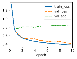
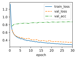
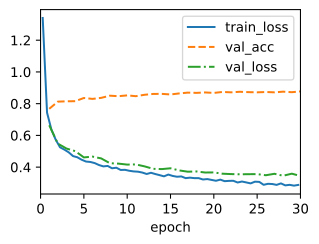
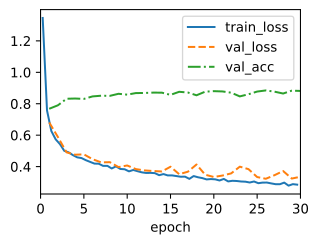
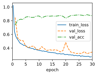
In the displayed run, validation accuracy settles near \(0.87\), above the earlier softmax-regression run. This comparison is illustrative: initialization, shuffling, framework defaults, and optimization settings also affect the result.
4.2.2 Concise Implementation
High-level framework layers provide a more concise implementation of the same architecture.
4.2.2.1 Model
Compared with our concise implementation of softmax regression (Section 3.5), the only difference is that we add two fully connected layers where we previously added only one. The first is the hidden layer, the second is the output layer.
class MLP(d2l.Classifier):
    def __init__(self, num_outputs, num_hiddens, lr):
        super().__init__()
        self.save_hyperparameters()
        self.net = nn.Sequential(nn.Flatten(), nn.LazyLinear(num_hiddens),
                                 nn.ReLU(), nn.LazyLinear(num_outputs))
class MLP(d2l.Classifier):
def __init__(self, num_outputs, num_hiddens, lr):
super().__init__()
self.save_hyperparameters()
self.net = tf.keras.models.Sequential([
tf.keras.layers.Flatten(),
tf.keras.layers.Dense(num_hiddens, activation='relu'),
tf.keras.layers.Dense(num_outputs)])class MLP(d2l.Classifier):
def __init__(self, num_outputs, num_hiddens, lr, num_inputs=784,
rngs=None):
super().__init__()
self.save_hyperparameters(ignore=['rngs'])
rngs = nnx.Rngs(d2l.get_key()) if rngs is None else rngs
self.hidden = nnx.Linear(num_inputs, num_hiddens, rngs=rngs)
self.output = nnx.Linear(num_hiddens, num_outputs, rngs=rngs)
def forward(self, X):
X = X.reshape((X.shape[0], -1)) # Flatten
return self.output(nnx.relu(self.hidden(X)))class MLP(d2l.Classifier):
def __init__(self, num_outputs, num_hiddens, lr):
super().__init__()
self.save_hyperparameters()
self.net = nn.Sequential()
self.net.add(nn.Dense(num_hiddens, activation='relu'),
nn.Dense(num_outputs))
self.net.initialize()A forward method applies each model transformation to the output of the preceding one. Here, MLP inherits the Module implementation (Section 2.2.2), which invokes self.net(X). The Sequential container applies its registered transformations in order and therefore defines the forward computation. Section 5.1.2 examines this container in detail.
4.2.2.2 Training
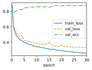
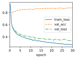
The training loop is the same as for softmax regression. This modularity enables us to separate matters concerning the model architecture from orthogonal considerations. Note that while the two versions compute the same architecture, they do not start from the same parameters: the scratch model draws its weights from \(\mathcal{N}(0, 0.01^2)\), whereas the concise version uses the library’s default initializer. Defaults differ across libraries and layer types, so the two versions need not start at comparable scales. Their training trajectories and final accuracies can therefore differ.
model = MLP(num_outputs=10, num_hiddens=256, lr=0.1)
trainer.fit(model, data)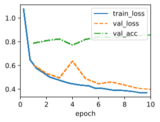
4.2.3 Summary
We have built and trained a multilayer perceptron in both from-scratch and concise forms. The from-scratch version exposes two weight matrices, two bias vectors, a ReLU, and the two affine computations. The concise version represents the same architecture as a four-element nn.Sequential stack. The training loop, loss, and data loader remain unchanged from softmax regression.
The from-scratch version also shows why high-level containers are useful: manually naming and tracking parameters becomes cumbersome as layers are added or reordered. nn.Sequential handles both registration and execution order.
Three questions remain open, and each is the subject of one of the next sections:
- How do gradients flow through this stack, and what can go wrong as it gets deeper? (Section 4.3, Section 4.4)
- Why does such a flexible model generalize to unseen data at all? (Section 4.5)
- How can we regularize it to generalize better? (Section 4.6)
The following sections address these requirements for reliable training.
4.2.4 Exercises
- Change the number of hidden units
num_hiddensand plot how its number affects the accuracy of the model. What is the best value of this hyperparameter? - Try adding a hidden layer to see how it affects the results. In particular, add one to the from-scratch model while keeping its \(\sigma = 0.01\) Gaussian initialization: you may find that the deeper network trains worse. Why that happens, and what to do about it, is the subject of Section 4.4.
- Why is it a bad idea to insert a hidden layer with a single neuron? What could go wrong?
- How does changing the learning rate alter your results? With all other parameters fixed, which learning rate gives you the best results? How does this relate to the number of epochs?
- Optimize all hyperparameters jointly: learning rate, number of epochs, number of hidden layers, and number of hidden units per layer.
- What is the best result you can get by optimizing over all of them?
- Why is it much more challenging to tune multiple hyperparameters?
- Describe an efficient strategy for optimizing over multiple parameters jointly.
- Compare the speed of the framework and the from-scratch implementation for a challenging problem. How does it change with the complexity of the network?
- Measure the speed of tensor–matrix multiplications for well-aligned and misaligned matrices. For instance, test for matrices with dimension 1024, 1025, 1026, 1028, and 1032.
- How does this change between GPUs and CPUs?
- Determine the memory bus width of your CPU and GPU.
- Try out different activation functions. Which one works best on Fashion-MNIST? Compare at least ReLU, tanh, sigmoid, and GELU (
torch.nn.functional.geluin PyTorch,jax.nn.geluin JAX). (Hint: for sigmoid and tanh you may need to retune the learning rate.) GELU is used in BERT and GPT-2-style Transformers, while many recent language models use gated SiLU/SwiGLU blocks. Does this small image task provide enough evidence to choose among them for a Transformer? - Compare the effect of three initialization scales on training: (a) small Gaussian noise with \(\sigma = 0.001\); (b) the value used in this section, \(\sigma = 0.01\); (c) large Gaussian noise with \(\sigma = 0.1\). Plot the training and validation curves for each. Why does \(\sigma\) matter? (Hint: consider what happens to the activations on the very first forward pass.) The principled answer is developed in Section 4.4.