%matplotlib inline
from d2l import torch as d2l
import torch
import numpy as onp # plain NumPy for the permutation test and bootstrap below27.5 Statistics
A model is fitted to a finite random sample, so its accuracy, learned weights, and other estimates would change if the data were sampled again. Statistics quantifies this variation. This section defines estimators and their bias and variance, then derives the bias–variance decomposition used to analyze underfitting and overfitting in Section 2.6. Hypothesis tests compare an observed difference with sampling variation, while confidence intervals report a range of parameter values compatible with an estimate. We write the unknown parameter \(\theta\) as a scalar; the vector case replaces squares by squared norms.
We use the following imports throughout the section, plus plain NumPy as onp for the label-shuffling in the permutation test and the resampling in the bootstrap.
%matplotlib inline
from d2l import tensorflow as d2l
import tensorflow as tf
import numpy as onp # plain NumPy for the permutation test and bootstrap below%matplotlib inline
from d2l import jax as d2l
import jax
from jax import numpy as jnp
import numpy as onp # plain NumPy for the permutation test and bootstrap below%matplotlib inline
from d2l import mxnet as d2l
from mxnet import np, npx
npx.set_np()
import numpy as onp # plain NumPy for the permutation test and bootstrap below27.5.1 Estimators and Their Quality
27.5.1.1 Estimators
An estimator is a rule that turns data into a value intended to estimate an unknown parameter. Given observations \(x_1,\ldots,x_n\), write
\[ \hat\theta_n = \hat f(x_1,\ldots,x_n) \]
The Bernoulli sample proportion and the Gaussian sample mean are examples from Section 27.3. Because the sample is random, \(\hat\theta_n\) is a random variable. Its distribution over repeated samples is the sampling distribution.
The main quality criteria answer different questions:
| Criterion | Question |
|---|---|
| Bias | Where is the sampling distribution centered relative to \(\theta\)? |
| Variance / standard error | How widely does the estimate vary across samples? |
| Mean squared error | How large is the squared error, combining bias and variance? |
| Consistency | Does the estimate approach \(\theta\) as \(n\) grows? |
| Efficiency | Within a specified estimator class, how small is its variance? |
27.5.1.2 Bias and Variance
The first feature is the center. The bias of \(\hat\theta_n\) measures the systematic gap between where the estimator centers and the truth,
\[ \operatorname{Bias}(\hat\theta_n) = \mathbb{E}[\hat\theta_n] - \theta , \tag{27.5.1}\]
the expectation taken over the random sample. When \(\operatorname{Bias}(\hat\theta_n)=0\) for every \(\theta\), the estimator is unbiased. Bias describes systematic error at a fixed sample size; it may persist or vanish as \(n\) grows.
The second feature is the spread. The variance measures how much the estimator fluctuates around its own center, with the standard error its square root,
\[ \operatorname{Var}(\hat\theta_n) = \mathbb{E}\!\left[(\hat\theta_n - \mathbb{E}[\hat\theta_n])^2\right], \qquad \operatorname{se}(\hat\theta_n) = \sqrt{\operatorname{Var}(\hat\theta_n)} . \tag{27.5.2}\]
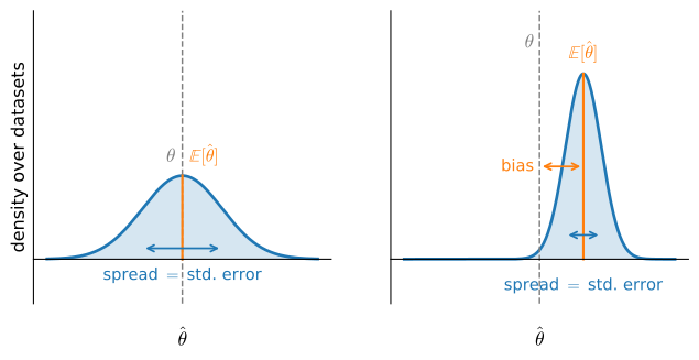
Note carefully that variance is measured against \(\mathbb{E}[\hat\theta_n]\), not against the true \(\theta\): it captures the noise in the estimator, not its accuracy. Figure 27.5.1 makes the two features visible by drawing the sampling distribution for two estimators of the same \(\theta\). Bias is the offset of the distribution’s center from \(\theta\); variance is its width.
27.5.1.3 Consistency and Efficiency
Bias and variance describe an estimator at a fixed sample size. Two further notions describe how it behaves as data accumulates. An estimator is asymptotically unbiased if its bias vanishes in the limit, \(\lim_{n\to\infty}\operatorname{Bias}(\hat\theta_n)=0\); many estimators used in practice are biased at finite \(n\) but asymptotically unbiased, which is usually good enough. A stronger and more useful guarantee is consistency: \(\hat\theta_n\) is consistent if it converges in probability to \(\theta\),
\[ \hat\theta_n \xrightarrow{P} \theta, \qquad\textrm{i.e.}\qquad P\bigl(|\hat\theta_n-\theta|>\varepsilon\bigr)\to 0 \quad\textrm{for every } \varepsilon>0 . \]
The weak law of large numbers gives the prototype: the sample mean is a consistent estimator of the population mean. A sufficient condition for consistency is that both bias and variance tend to zero. The conditions are separate: asymptotic unbiasedness does not imply consistency if variance persists, and vanishing variance does not repair persistent bias.
Finally, efficiency compares variance within a specified estimator class. For regular scalar models, the Cramér–Rao bound in Section 27.3 gives the floor \(1/(nI(\theta))\) for unbiased estimators under its assumptions. The MLE attains this floor asymptotically in regular models. Efficiency alone does not rank biased estimators; mean squared error does.
27.5.2 The Bias-Variance Decomposition
We now have two distinct ways an estimator can be wrong, a systematic offset (bias) and random fluctuation (variance), and a single number that ought to combine them: the mean squared error. The MSE is exactly the sum of these two contributions, with no cross term.
27.5.2.1 Mean Squared Error and the Decomposition
The simplest summary of how far an estimator lands from the truth is the mean squared error,
\[ \operatorname{MSE}(\hat\theta_n) = \mathbb{E}\!\left[(\hat\theta_n-\theta)^2\right] . \tag{27.5.3}\]
It is always non-negative, and the smaller it is the closer \(\hat\theta_n\) sits to \(\theta\) on average. If you have read Section 2.1 you will recognize it as the squared-error loss, now applied to an estimator rather than a prediction.
Proposition (bias-variance decomposition). For any estimator \(\hat\theta_n\) of a fixed parameter \(\theta\),
\[ \operatorname{MSE}(\hat\theta_n) = \operatorname{Bias}(\hat\theta_n)^2 + \operatorname{Var}(\hat\theta_n) . \tag{27.5.4}\]
Proof. Abbreviate \(\mu = \mathbb{E}[\hat\theta_n]\), the center of the estimator, and add and subtract it inside the square:
\[ \operatorname{MSE}(\hat\theta_n) = \mathbb{E}\!\left[(\hat\theta_n - \theta)^2\right] = \mathbb{E}\!\left[\bigl((\hat\theta_n - \mu) + (\mu - \theta)\bigr)^2\right]. \]
Expanding the square gives three terms. The first is \(\mathbb{E}[(\hat\theta_n-\mu)^2]=\operatorname{Var}(\hat\theta_n)\); the last is \((\mu-\theta)^2=\operatorname{Bias}(\hat\theta_n)^2\), a constant. The middle, cross term vanishes, because \(\mu-\theta\) is a constant and \(\hat\theta_n-\mu\) has mean zero by the definition of \(\mu\):
\[ 2\,(\mu-\theta)\,\mathbb{E}[\hat\theta_n - \mu] = 2\,(\mu-\theta)\,(\mu - \mu) = 0 . \]
What remains is \(\operatorname{Var}(\hat\theta_n)+\operatorname{Bias}(\hat\theta_n)^2\). \(\blacksquare\)
Because the centered fluctuation has mean zero, its cross term with the bias vanishes, giving the decomposition in Figure 27.5.1. This identity also supplies a consistency criterion. If both \(\operatorname{Bias}(\hat\theta_n)\to0\) and \(\operatorname{Var}(\hat\theta_n)\to0\), then Equation 27.5.4 implies \(\operatorname{MSE}(\hat\theta_n)\to0\). Markov’s inequality applied to \((\hat\theta_n-\theta)^2\) then gives \[ P(|\hat\theta_n-\theta|>\varepsilon) \le \frac{\operatorname{MSE}(\hat\theta_n)}{\varepsilon^2}\to0, \] so \(\hat\theta_n\xrightarrow{P}\theta\). For an unbiased estimator this reduces to Chebyshev’s inequality. The concentration results in Section 27.6 provide sharper rates for bounded or sub-Gaussian observations.
27.5.2.2 The Law of Large Numbers
Assembling the pieces just derived yields the guarantee promised above, the same one that Section 25.4 invoked to justify Monte Carlo integration.
Proposition (weak law of large numbers). If \(x_1,\ldots,x_n\) are i.i.d. with mean \(\mu\) and finite variance \(\sigma^2\), the sample mean \(\bar x_n = \frac1n\sum_{i=1}^n x_i\) converges in probability to \(\mu\):
\[ \bar x_n \xrightarrow{P} \mu , \qquad\textrm{indeed}\qquad P\bigl(|\bar x_n - \mu| > \varepsilon\bigr) \le \frac{\sigma^2}{n\,\varepsilon^2} \quad\textrm{for every } \varepsilon > 0 . \tag{27.5.5}\]
Proof. The sample mean is unbiased, \(\mathbb{E}[\bar x_n]=\mu\), by linearity of expectation, and its variance is \(\operatorname{Var}(\bar x_n)=\sigma^2/n\) by the variance of a sum of independent variables (Section 27.1). By Equation 27.5.4 its MSE is therefore \(0 + \sigma^2/n\), and the Markov step above turns that into the displayed bound, which vanishes as \(n\to\infty\). \(\blacksquare\)
Finite variance is more than the theorem needs: a finite mean \(\mathbb{E}|x_1|<\infty\) already suffices, at the cost of a longer argument (Wasserman 2013). In whichever form, this is the law that makes averaging work: it is why a Monte Carlo estimate of an integral converges, why a test-set accuracy estimates the true error rate, and why the empirical loss a model is trained on tracks the expected loss it is meant to minimize.
27.5.2.3 The Trade-off and Generalization
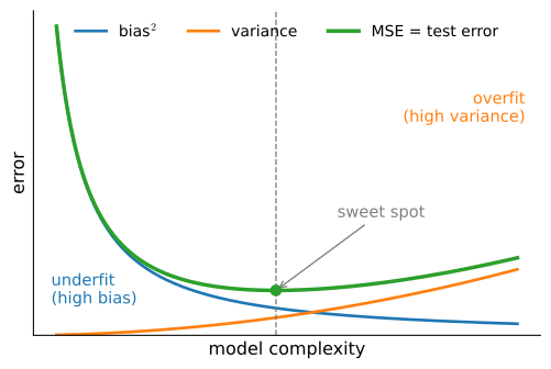
For squared-error prediction, the same decomposition separates error due to the fitted predictor’s bias, its sampling variance, and irreducible label noise (Geman et al. 1992). In many classical model sequences, greater flexibility lowers bias and raises variance, producing the U-shaped curve in Figure 27.5.2. Regularization can improve risk by accepting more bias in exchange for less variance. This U-shape is a common pattern, not a theorem about every model sequence; interpolating models can exhibit double descent (Section 27.6).
27.5.2.4 The Decomposition in Code
The decomposition is an exact algebraic identity, so it should hold to numerical precision on a concrete example. We first define bias and MSE as the formulas Equation 27.5.1 and Equation 27.5.3 say: averages over a collection of estimates, against the true parameter.
import numpy as onp
def stat_bias(true_theta, est_theta):  # E[theta_hat] - theta
    return onp.mean(est_theta) - true_theta

def mse(est_theta, true_theta):        # E[(theta_hat - theta)^2]
    return onp.mean(onp.square(est_theta - true_theta))
To exercise these we need the sampling distribution itself, not a single dataset: we draw many independent datasets from \(\mathcal{N}(\theta,\sigma^2)\), compute the sample mean on each, and collect the resulting estimates. Their spread is the variance and their center the bias.
import numpy as onp
theta_true, sigma = 1.0, 4.0
num_datasets, n = 10000, 30  # 10k datasets, each of n=30 points
samples = onp.random.normal(theta_true, sigma, (num_datasets, n))
theta_hats = samples.mean(axis=1)  # one sample-mean estimate per dataset
Now we read the decomposition off the empirical sampling distribution: the MSE of the estimates around the true \(\theta\) should match the squared bias plus the variance of the estimates around their own mean, the two sides of Equation 27.5.4. One detail matters for exactness. The identity is a statement about expectations under a single distribution, here the empirical distribution of our \(10{,}000\) estimates, whose expectations are plain averages. That forces the plug-in variance, which divides by the number of estimates (ddof=0, the default in most libraries), rather than the unbiased \(n-1\) variant we meet in the next subsection. With the plug-in choice the proof’s algebra goes through verbatim for the empirical averages.
import numpy as onp
bias = stat_bias(theta_true, theta_hats)
# Default ddof=0: the plug-in variance of the estimates, which makes the
# identity exact for empirical averages (the n-1 variant is the next subsection)
var = onp.var(theta_hats)
mse(theta_hats, theta_true), var + onp.square(bias)(np.float64(0.5280212902905295), np.float64(0.5280212902905296))(np.float64(0.5378135196239607), np.float64(0.5378135196239607))(np.float64(0.5388513183973679), np.float64(0.538851318397368))(0.5424464736414311, 0.5424464736414311)The two numbers agree to floating-point round-off (the identity is exact), and both are close to the theoretical value. For the sample mean of \(\mathcal{N}(\theta,\sigma^2)\) the bias is exactly zero (the average of unbiased draws is unbiased) and the variance is \(\sigma^2/n\) (the variance-of-a-sum result from Section 27.1), so \(\operatorname{MSE}=\sigma^2/n = 16/30 \approx 0.53\). Because both the bias (\(0\)) and the variance (\(\sigma^2/n\to0\)) vanish as \(n\to\infty\), the sample mean is consistent, exactly as the weak law of large numbers Equation 27.5.5 asserts: the simulation is that proposition run in the small.
27.5.2.5 Why the Unbiased Variance Divides by \(n-1\)
The sample mean was unbiased for free. The sample variance is more delicate, and it exposes a subtlety that the library’s std function encodes in a ddof flag. Given samples \(x_1,\ldots,x_n\) with sample mean \(\bar x=\frac1n\sum_i x_i\), the natural estimator of the population variance \(\sigma^2\) would average the squared deviations,
\[ s_0^2 = \frac1n\sum_{i=1}^n (x_i-\bar x)^2 . \]
This estimator is biased downward because its deviations are measured from the sample mean \(\bar x\), which minimizes the sum of squared deviations for the observed sample, rather than from the unknown population mean \(\mu\). The estimator \(s_0^2\) is also the Gaussian maximum-likelihood estimate of variance, so this calculation exhibits the finite-sample bias discussed in Section 27.3. Dividing by \(n-1\) instead of \(n\) removes the bias.
Proposition (unbiased sample variance). For i.i.d. samples with variance \(\sigma^2\),
\[ s^2 = \frac{1}{n-1}\sum_{i=1}^n (x_i-\bar x)^2 \qquad\textrm{satisfies}\qquad \mathbb{E}[s^2] = \sigma^2 . \tag{27.5.6}\]
Proof. Center the data at the true mean \(\mu\) by writing \(x_i-\bar x = (x_i-\mu)-(\bar x-\mu)\), and expand the sum of squared deviations:
\[ \sum_{i=1}^n (x_i-\bar x)^2 = \sum_{i=1}^n (x_i-\mu)^2 - n\,(\bar x-\mu)^2 , \]
where the cross term collapsed because \(\sum_i (x_i-\mu) = n(\bar x-\mu)\). Now take expectations. Each \(\mathbb{E}[(x_i-\mu)^2]=\sigma^2\), so the first sum has expectation \(n\sigma^2\). The second uses the variance of the sample mean, \(\mathbb{E}[(\bar x-\mu)^2]=\operatorname{Var}(\bar x)=\sigma^2/n\), so that term has expectation \(n\cdot\sigma^2/n=\sigma^2\). Hence
\[ \mathbb{E}\!\left[\sum_{i=1}^n (x_i-\bar x)^2\right] = n\sigma^2 - \sigma^2 = (n-1)\,\sigma^2 . \]
Dividing by \(n-1\) gives \(\mathbb{E}[s^2]=\sigma^2\). \(\blacksquare\)
The intuition is degrees of freedom: estimating \(\bar x\) from the same data consumes one degree of freedom, so only \(n-1\) of the deviations are free to vary, and dividing by \(n-1\) rather than \(n\) corrects for it exactly. (As \(n\to\infty\) the two estimators agree, so \(s_0^2\) is biased but asymptotically unbiased and consistent.) We can watch the bias appear and the correction remove it by estimating both variances over many datasets and averaging.
import numpy as onp
n = 3  # small n makes the 1/n bias glaring; the gap shrinks like 1/n
data = onp.random.normal(0, 2, (100000, n))  # sigma^2 = 4
dev2 = onp.square(data - data.mean(axis=1, keepdims=True)).sum(axis=1)
print('true variance    = 4')
print(f'E[divide by n]   = {float((dev2 / n).mean()):.3f}  (biased)')
print(f'E[divide by n-1] = {float((dev2 / (n - 1)).mean()):.3f} (unbiased)')true variance = 4
E[divide by n] = 2.663 (biased)
E[divide by n-1] = 3.994 (unbiased)true variance = 4
E[divide by n] = 2.669 (biased)
E[divide by n-1] = 4.004 (unbiased)true variance = 4
E[divide by n] = 2.684 (biased)
E[divide by n-1] = 4.026 (unbiased)true variance = 4
E[divide by n] = 2.670 (biased)
E[divide by n-1] = 4.004 (unbiased)With \(n=3\) the biased estimator averages near \(\tfrac{n-1}{n}\sigma^2 = \tfrac23\cdot 4 \approx 2.67\), while dividing by \(n-1\) recovers \(4\), confirming Equation 27.5.6. The ddof argument (“delta degrees of freedom”) selects the denominator: ddof=1 divides by \(n-1\), ddof=0 by \(n\).
27.5.3 Hypothesis Testing
Bias and variance characterize the error of an estimator. Hypothesis testing addresses a different question: whether an observed difference between two groups or models is compatible with sampling variation under a specified null hypothesis. This framework underlies A/B tests and benchmark comparisons.
27.5.3.1 Null and Alternative Hypotheses
A hypothesis test weighs evidence against a default claim. The null hypothesis \(H_0\) is that default, typically “there is no effect” (e.g. the new model is no better than the baseline), and the alternative \(H_A\) is the effect we hope to detect: sometimes the null’s outright negation, but often one-sided or otherwise composite, e.g. “the new model is better.” The asymmetry is deliberate: we never prove \(H_0\); we either gather enough evidence to reject it in favor of \(H_A\), or we fail to, much as a court returns “guilty” or “not guilty” rather than “innocent.”
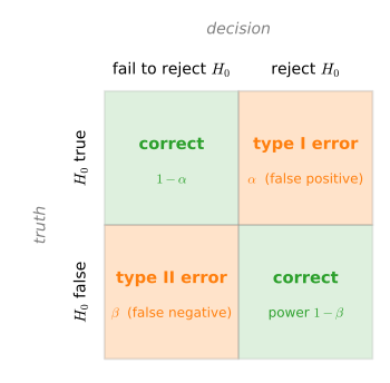
Because the data are random, the decision can go wrong in two ways. A type I error (false positive) is rejecting \(H_0\) when it is in fact true: declaring an effect that is not there. A type II error (false negative) is failing to reject \(H_0\) when it is in fact false: missing a real effect. Their rates have standard names, the significance level \(\alpha\) and \(\beta\),
\[ \alpha = P(\textrm{reject } H_0 \mid H_0 \textrm{ true}), \qquad \beta = P(\textrm{fail to reject } H_0 \mid H_0 \textrm{ false}), \]
and the four possible outcomes arrange into the \(2\times2\) decision matrix of Figure 27.5.3: rows are whether \(H_0\) is true or false, columns are our decision. The diagonal cells are correct; the off-diagonal cells are the two errors. One caveat on the notation: when \(H_A\) is composite, “\(H_0\) false” does not pin down a single distribution, so \(\beta\) (and the power below) is a function of the true parameter, evaluated at a given alternative; that is exactly how Figure 27.5.4 will draw it.
27.5.3.2 Significance and Power
We choose the type I error rate up front: the significance level \(\alpha\) is the risk of a false positive we are willing to tolerate, conventionally \(\alpha=0.05\). The complement \(1-\alpha\) is the confidence level, the name that returns with the confidence intervals below. The bottom-right cell of the matrix is the quantity we want to be large: the statistical power
\[ 1 - \beta = P(\textrm{reject } H_0 \mid H_0 \textrm{ false}) \]
is the probability the test detects a real effect, again evaluated at a given alternative. A test with \(\alpha=0.05\) but power \(0.2\) rejects a true null only \(5\%\) of the time yet still misses \(80\%\) of genuine effects of that size: underpowered, and useless for confirming improvements. A common target is \(1-\beta=0.8\).
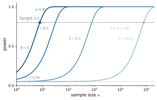
Power is what determines how much data we need, and the simplest test of all makes the accounting explicit. In the one-sample two-sided \(z\)-test the data are Gaussian with known variance \(\sigma^2\), the null is \(H_0\!:\mu=0\), the statistic is \(T=\sqrt n\,\bar x/\sigma\), which under \(H_0\) is exactly standard normal, and we reject when \(|T|\ge z_{1-\alpha/2}\), where \(z_q\) denotes the standard-normal quantile (\(z_{0.975}\approx1.960\) at \(\alpha=0.05\)). Now suppose the true mean is some \(\mu\neq0\) and write \(\delta=|\mu|/\sigma\) for the standardized effect, the size of the effect measured in units of the noise. Then \(T\) is Gaussian with mean \(\pm\delta\sqrt n\) and unit variance, so the test detects the effect with probability \(\Phi(\delta\sqrt n - z_{1-\alpha/2})\), where \(\Phi\) is the standard-normal c.d.f. (the far tail on the opposite side contributes negligibly). Setting this power equal to \(1-\beta\), so that \(\delta\sqrt n - z_{1-\alpha/2} = z_{1-\beta}\), and solving for \(n\) gives the sample size needed to detect a standardized effect \(\delta\) at level \(\alpha\) with power \(1-\beta\):
\[ n \;=\; \frac{\bigl(z_{1-\alpha/2} + z_{1-\beta}\bigr)^{2}}{\delta^{2}} . \tag{27.5.7}\]
For \(\alpha=0.05\) and power \(0.8\), \(z_{0.975}\approx1.960\) and \(z_{0.8}\approx0.842\), giving \(n\approx7.85/\delta^2\). Thus an effect of one standard deviation requires about eight samples, whereas an effect of \(0.01\) standard deviations requires about 78,489. Figure 27.5.4 plots the corresponding power curves. For each nonzero effect, power approaches one as \(n\) increases and reaches \(0.8\) at a sample size proportional to \(1/\delta^2\). At \(\delta=0\), rejection occurs with probability \(\alpha\), the test’s false-positive rate.
27.5.3.3 Test Statistics, \(p\)-values, and Significance
To run a test we compress the data into a single test statistic \(T(x)\), a scalar chosen so that extreme values are unlikely under \(H_0\); the mean difference between two groups is a natural choice. Under \(H_0\) the statistic has a known (often approximately Gaussian) null distribution, which is what lets us judge whether an observed value is surprising.
The verdict is delivered by the \(p\)-value: the probability, computed under \(H_0\), of seeing a statistic at least as extreme as the one we observed. For a two-sided test (the common case, where a deviation in either direction counts as evidence),
\[ p\textrm{-value} = P_{H_0}\bigl(|T(X)| \ge |T(x)|\bigr), \]
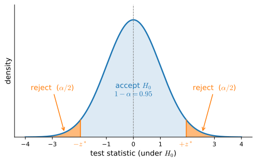
valid when the null distribution is symmetric about \(0\); in general the two-sided \(p\)-value is \(2\,\min\{P_{H_0}(T\ge t),\, P_{H_0}(T\le t)\}\), which doubles the smaller tail. The one-sided version uses a single tail. We reject \(H_0\) when \(p \le \alpha\). Geometrically, the rejection region is the set of statistic values whose \(p\)-value falls below \(\alpha\); Figure 27.5.5 shows it for a Gaussian null at \(\alpha=0.05\) as the two tails beyond the critical values \(\pm 1.96\) (the \(z\)-test’s rejection region \(|T|\ge1.96\) from above), together holding \(5\%\) of the probability. A statistic landing in those tails would be very unlikely if \(H_0\) held, so we reject.
A persistent warning is in order, because the \(p\)-value is among the most misread numbers in science (Wasserstein and Lazar 2016). It is \(P(\textrm{data this extreme}\mid H_0)\), a statement about the data given the null; it is not \(P(H_0\mid\textrm{data})\), the probability the null is true, which would require a prior and Bayes’ rule. A large \(p\)-value does not confirm \(H_0\); it means only that we failed to detect an effect, possibly because the test was underpowered.
A subtler trap is multiple testing. The \(\alpha=0.05\) guarantee holds for a single pre-specified test; run \(m\) of them under a true null (sweeping hyperparameters, comparing across benchmarks, retrying until something “works”) and the chance of at least one spurious win is \(1-(1-\alpha)^m\), which already exceeds \(0.4\) at \(m=10\). Reporting only the test that cleared \(p\le\alpha\) is \(p\)-hacking, and it is how noise gets published as a result. The simplest guard is the Bonferroni correction (Bonferroni 1936): to hold the family-wide false-positive rate at \(\alpha\), test each of the \(m\) hypotheses at the stricter level \(\alpha/m\). When \(m\) runs into the hundreds or thousands, as in a hyperparameter sweep or a screen of model variants, Bonferroni grows hopelessly conservative, and large-scale practice instead controls the false discovery rate, the expected fraction of rejections that are false, via the Benjamini–Hochberg procedure (Benjamini and Hochberg 1995), which sorts the \(m\) \(p\)-values in increasing order and rejects the \(k\) smallest, with \(k\) the largest index satisfying \(p_{(k)}\le k\alpha/m\).
To summarize, a hypothesis test proceeds in five steps:
- State \(H_0\) and \(H_A\).
- Fix the significance level \(\alpha\) and a target power \(1-\beta\) (which, with the expected effect size, sets the sample size).
- Collect the data.
- Compute the test statistic and its \(p\)-value under \(H_0\).
- Reject \(H_0\) if \(p \le \alpha\); otherwise fail to reject.
27.5.3.4 Comparing Two Models
Let us walk through the five steps once, on the comparison practitioners face most often: is model B really better than model A, or did it just draw lucky seeds? We simulate per-seed test accuracies for the two models: twenty training runs each, with a true gap of \(0.8\%\) buried in seed-to-seed noise of comparable size. Step 1: \(H_0\) is that the two models are equally good, i.e. the two accuracy samples come from the same distribution, and \(H_A\) is that they differ; step 2: \(\alpha=0.05\). The test statistic is the gap between the mean accuracies. Rather than assume a Gaussian null distribution, we use a permutation test (Fisher 1935), which manufactures the null distribution from the data itself: if \(H_0\) holds, the labels “A” and “B” carry no information (the \(40\) numbers are exchangeable), so shuffling the labels and recomputing the gap, many times over, shows exactly how large a gap arises by pure chance. The two-sided \(p\)-value is the fraction of shuffles producing a gap at least as extreme as the observed one (counting the observed labeling itself among them, which keeps the estimate valid and never exactly zero).
rng = onp.random.default_rng(1)
num_seeds = 20                               # 20 training runs per model
acc_a = rng.normal(0.850, 0.010, num_seeds)  # per-seed accuracy, model A
acc_b = rng.normal(0.858, 0.010, num_seeds)  # model B: a real +0.008 gap
observed = acc_b.mean() - acc_a.mean()       # test statistic: gap in means

pooled = onp.concatenate([acc_a, acc_b])     # under H_0 the labels are arbitrary
B = 10000
gaps = onp.empty(B)
for b in range(B):
    perm = rng.permutation(pooled)           # shuffle the model labels
    gaps[b] = perm[num_seeds:].mean() - perm[:num_seeds].mean()
p_value = (1 + (onp.abs(gaps) >= abs(observed)).sum()) / (B + 1)  # two-sided
print(f'observed gap        = {observed:.4f}')
print(f'permutation p-value = {p_value:.4f}')

d2l.set_figsize()
d2l.plt.hist(gaps, bins=50, color='#1f77b4', alpha=0.8)
d2l.plt.axvline(observed, color='#ff7f0e', lw=2)      # the observed gap
d2l.plt.axvline(-observed, color='#ff7f0e', lw=2, ls='--')
d2l.plt.xlabel('gap under label shuffling')
d2l.plt.ylabel('count');observed gap = 0.0073
permutation p-value = 0.0197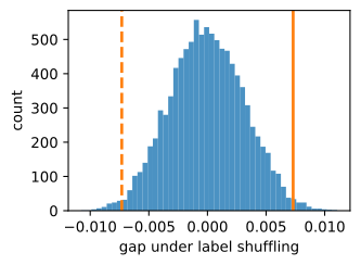
observed gap        = 0.0073
permutation p-value = 0.0197
observed gap        = 0.0073
permutation p-value = 0.0197
observed gap        = 0.0073
permutation p-value = 0.0197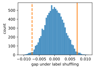
The observed difference is \(0.0073\): model B is better by about 0.73 percentage points. Only about 2% of label permutations produce a difference at least this large in magnitude, so \(p\approx0.02\le\alpha=0.05\) and the test rejects \(H_0\).
The permutation distribution is approximately bell-shaped around zero. This shape is not assumed by the test; it follows here from a finite-population central limit effect for means formed from the pooled 40 observations, related to the iid CLT in Section 27.2. The observed statistic lies in its tail. The result is nevertheless close to the threshold: an improvement of about 0.8 percentage points is detected with 20 seeds but would often be missed with five. A permutation test requires exchangeability under the null, not Gaussian observations, and can be applied to other group-comparison statistics.
One refinement matters in practice. When the comparison is paired, with models A and B trained and evaluated on the same seeds, the exchangeable objects are not the \(40\) pooled numbers but the per-seed differences, and the right test flips the sign of each difference at random: the paired, or sign-flip, permutation test. It respects the pairing and typically gains power.
27.5.4 Confidence Intervals
A point estimate \(\hat\theta\) does not describe its sampling uncertainty. A confidence interval is constructed by a procedure designed to cover the fixed parameter \(\theta\) at a specified long-run rate (Neyman 1937).
27.5.4.1 Definition and Interpretation
A confidence interval for \(\theta\) is an interval \(C_n\) computed from the data such that
\[ P_\theta(C_n \ni \theta) \ge 1 - \alpha \quad \textrm{for all } \theta, \tag{27.5.8}\]
where \(1-\alpha\) is the confidence level or coverage. We write \(C_n \ni \theta\) rather than \(\theta \in C_n\) to stress where the randomness lives: \(\theta\) is a fixed unknown, and it is the interval \(C_n\) that is random, redrawn with every dataset.
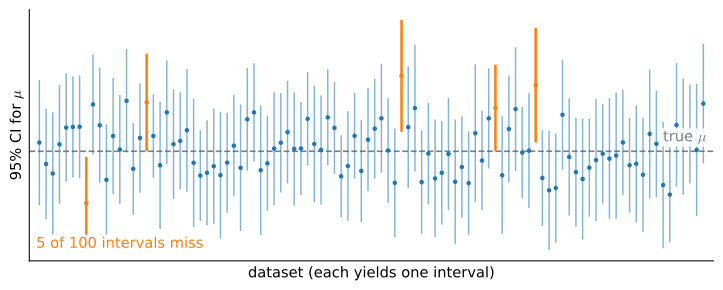
A 95% confidence interval does not assign probability 0.95 to the fixed parameter lying in the realized interval. Instead, under repeated sampling, 95% of intervals constructed by the procedure contain \(\theta\). Figure 27.5.6 illustrates this interpretation with 100 independent datasets: most intervals contain the fixed parameter and some do not.
A Bayesian credible interval has a different interpretation because \(\theta\) is assigned a posterior distribution conditional on a prior and the observed data. For the Beta posterior in Section 27.2, a 95% credible interval for a Bernoulli parameter is given by the 2.5% and 97.5% posterior quantiles of \(\mathrm{Beta}(\alpha+x,\beta+n-x)\). Its probability statement is conditional on the chosen model and prior.
27.5.4.2 A Gaussian Example
The classic case is the mean of a Gaussian \(\mathcal{N}(\mu,\sigma^2)\) with both parameters unknown. From \(n\) samples we form the usual estimators \(\hat\mu_n=\frac1n\sum_i x_i\) and the unbiased \(\hat\sigma_n^2=\frac1{n-1}\sum_i (x_i-\hat\mu_n)^2\) from Equation 27.5.6. The studentized statistic, centered and scaled by the estimated standard error \(\hat\sigma_n/\sqrt n\) in place of the unknown true one,
\[ T = \frac{\hat\mu_n - \mu}{\hat\sigma_n/\sqrt n} , \]
follows Student’s \(t\)-distribution on \(n-1\) degrees of freedom (Student (Gosset 1908), a fact we take on faith here; the distribution itself is constructed in Section 27.2. As \(n\to\infty\) the \(t\)-distribution approaches a standard Gaussian, and the attribution of that limit matters. For Gaussian data the numerator \(\hat\mu_n-\mu\) is exactly Gaussian at every \(n\); the limit comes from the denominator, since \(\hat\sigma_n\) is consistent for \(\sigma\) (the law of large numbers Equation 27.5.5 again, applied to squared deviations) and replacing a factor that converges in probability to a constant leaves a limiting distribution unchanged (Slutsky’s theorem, also taken on faith (Wasserman 2013)). The central limit theorem of Section 27.2 enters for non-Gaussian data: it makes the sampling distribution of the mean asymptotically Gaussian anyway, so the interval below remains asymptotically valid for the mean of any finite-variance distribution, which is why it gets used so freely in practice. For large \(n\), then, \(T\) lands in \([-1.96, 1.96]\) with probability \(\approx95\%\) (the Gaussian’s central \(95\%\)): exactly \(95\%\) in the Gaussian limit, and slightly less at finite \(n\), where the exact \(t\)-distribution has heavier tails and one should use the wider \(t\)-quantile in its place. Rearranging \(-1.96 \le T \le 1.96\) for \(\mu\) yields the interval
\[ \left[\hat\mu_n - 1.96\,\frac{\hat\sigma_n}{\sqrt n},\; \hat\mu_n + 1.96\,\frac{\hat\sigma_n}{\sqrt n}\right]. \tag{27.5.9}\]
This is one of the most-used formulas in statistics. The half-width \(1.96\,\hat\sigma_n/\sqrt n\) shrinks like \(1/\sqrt n\): to halve the interval we need four times the data. Let us construct one for a standard-normal sample, taking the asymptotic \(t_\star=1.96\).
import numpy as onp
N = 1000
samples = onp.random.normal(loc=0, scale=1, size=(N,))
t_star = 1.96  # asymptotic value; small N would look this up in a t-table
mu_hat = onp.mean(samples)
se = samples.std(ddof=1) / onp.sqrt(N)  # ddof=1: unbiased sigma_hat
(mu_hat - t_star * se, mu_hat + t_star * se)(np.float64(-0.024950383891352977), np.float64(0.09469291735831173))(np.float64(-0.13855897938953968), np.float64(-0.019010307571063846))(np.float64(-0.06592050600469802), np.float64(0.0572295754390227))(-0.05504203005451702, 0.06867651061262059)The interval is narrow and brackets the true mean \(0\), as it should roughly \(95\%\) of the time. The same \(1/\sqrt n\) scaling shows up everywhere uncertainty is reported (error bars on a learning curve, the spread of accuracies across random seeds), and Equation 27.5.9 is the formula behind them.
“Roughly \(95\%\) of the time” is the Neyman guarantee Equation 27.5.8, and we can audit it. The cell below repeats the whole procedure one thousand times: draw a fresh dataset, build the interval Equation 27.5.9, and check whether it traps the true mean. The hit count should land near \(950\).
rng = onp.random.default_rng(0)
mu, n, trials = 0.0, 100, 1000
data = rng.normal(mu, 1.0, (trials, n))           # one row = one fresh dataset
mu_hat = data.mean(axis=1)
se = data.std(axis=1, ddof=1) / onp.sqrt(n)
hits = (onp.abs(mu_hat - mu) <= 1.96 * se)        # interval traps the truth?
print(f'{hits.sum()} of {trials} intervals contain the true mean '
      f'(expected about {0.95 * trials:.0f})')
937 of 1000 intervals contain the true mean (expected about 950)This simulation obtains 937 covered intervals. For \(n=100\), using \(1.96\) in place of the exact \(t\) quantile gives true coverage of about 94.7%, or 947 intervals in expectation. The binomial standard deviation of the coverage count is about seven, so 937 is 1.4 standard deviations below its expectation and is consistent with sampling variation. This count is the repeated-sampling interpretation shown in Figure 27.5.6.
Propagating error bars: the delta method. Often the number we report is not \(\hat\theta\) itself but a smooth function of it: the log-odds of an accuracy, the ratio of two losses, a percentage change. A first-order Taylor expansion, \(g(\hat\theta)\approx g(\theta)+g'(\theta)\,(\hat\theta-\theta)\), says the fluctuation of \(g(\hat\theta)\) is the fluctuation of \(\hat\theta\) scaled by the local slope, so standard errors propagate as
\[ \operatorname{se}\bigl(g(\hat\theta)\bigr) \;\approx\; \bigl|g'(\hat\theta)\bigr|\,\operatorname{se}(\hat\theta), \tag{27.5.10}\]
the delta method (Wasserman 2013). For instance, an accuracy of \(\hat p=0.90\) measured on \(n=1{,}000\) test examples has \(\operatorname{se}(\hat p)=\sqrt{\hat p(1-\hat p)/n}\approx 0.0095\); reporting the log-odds \(g(\hat p)=\log\frac{\hat p}{1-\hat p}\) instead, the slope \(g'(\hat p)=1/(\hat p(1-\hat p))\approx 11.1\) stretches the error bar to \(\approx 0.105\) on the log-odds scale. The same rule with a gradient in place of \(g'\) handles vector parameters, and when no derivative is convenient the bootstrap below sidesteps the calculus entirely.
27.5.4.3 The Bootstrap
The Gaussian interval Equation 27.5.9 uses a closed-form standard error for the mean, \(\hat\sigma_n/\sqrt n\). For a median, correlation, test accuracy, AUC, or BLEU score, analytic sampling calculations may be unavailable or inconvenient. The bootstrap estimates them by simulation.
The bootstrap, introduced by Bradley Efron (Efron 1979), escapes this with a single substitution. We never had access to the true distribution \(F\) that generated our \(n\) data points; if we did, we could simulate the sampling distribution of a chosen statistic by drawing fresh datasets from \(F\) and recomputing it. The bootstrap’s move, the plug-in principle, is to substitute the empirical distribution \(\hat F_n\), which puts mass \(1/n\) on each observed point, for the unknown \(F\). Drawing \(n\) points from \(\hat F_n\) is exactly resampling our own data \(n\) times with replacement. Concretely:
- From the original sample of size \(n\), draw \(n\) points with replacement to form a bootstrap resample; some points appear several times, others not at all.
- Compute the statistic \(\hat\theta^*\) on the resample.
- Repeat \(B\) times to obtain \(\hat\theta^*_1,\ldots,\hat\theta^*_B\).
Standard error. The standard deviation of the \(B\) replicates estimates the standard error of \(\hat\theta\). A few hundred replicates can be adequate for a rough standard error; more are useful when Monte Carlo error matters.
Percentile interval. The empirical \(\alpha/2\) and \(1-\alpha/2\) quantiles of \(\{\hat\theta_b^*\}\) define the percentile interval. Tail quantiles require more replicates, commonly at least \(1{,}000\)–\(2{,}000\); the example uses \(B=10{,}000\). The percentile method is simple and transformation-equivariant, but it does not automatically correct bias or poor coverage caused by strong skewness. Basic, studentized, or bias-corrected and accelerated (BCa) intervals may be preferable when those effects matter.
Validity. The resampling distribution is centered near \(\hat\theta\), not the unknown \(\theta\), and estimates shape and width from one sample. The ordinary iid bootstrap is valid for many regular, sufficiently smooth statistics under iid sampling. It can fail for extrema, boundary parameters, very small samples, and nonsmooth or non-identifiable problems. Dependent or clustered observations require a block, cluster, or other structure-preserving bootstrap. Exercise 1 gives the classic failure for a sample maximum.
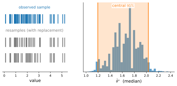
We now bootstrap the median of a skewed sample without using an analytic standard-error formula. A matrix of random indices draws all \(B\) resamples at once.
rng = onp.random.default_rng(0)
data = rng.exponential(scale=1.0, size=200)  # skewed: median != mean, no SE formula
n = len(data)
theta_hat = onp.median(data)                 # statistic of interest

B = 10000                                     # number of bootstrap resamples
idx = rng.integers(0, n, size=(B, n))         # n positions per resample, WITH replacement
boot = onp.median(data[idx], axis=1)          # one median per resample

se_boot = boot.std(ddof=1)                    # bootstrap standard error of the median
ci_pct = onp.percentile(boot, [2.5, 97.5])    # percentile 95% CI -- no formula needed
print(f'sample median        = {theta_hat:.3f}')
print(f'bootstrap SE         = {se_boot:.3f}')
print(f'percentile 95% CI    = ({ci_pct[0]:.3f}, {ci_pct[1]:.3f})')
sample median = 0.808
bootstrap SE = 0.072
percentile 95% CI = (0.682, 0.955)The calculation gives a bootstrap standard error and percentile interval for the median without a closed-form derivation. Its validity still rests on the regularity and iid-sampling conditions just stated. For contrast, the Gaussian formula Equation 27.5.9 targets the mean, a different quantity, which on this skewed sample lies above the median.
mu_hat = data.mean()
se_mean = data.std(ddof=1) / n**0.5           # closed-form SE, but only for the mean
ci_gauss = (mu_hat - 1.96 * se_mean, mu_hat + 1.96 * se_mean)
print(f'Gaussian 95% CI (mean) = ({ci_gauss[0]:.3f}, {ci_gauss[1]:.3f})')
Gaussian 95% CI (mean) = (0.986, 1.272)The two intervals answer different questions. The percentile interval for the median is slightly asymmetric about \(\hat\theta\) because it inherits the shape of the resampling distribution rather than imposing a symmetric Gaussian form. In machine-learning evaluations, a suitably designed bootstrap can estimate uncertainty for quantities such as held-out accuracy, AUC, or BLEU (Efron and Hastie 2016); the sampling unit and dependence structure must match the resampling scheme. Section 27.7 applies the iid version to test accuracy.
27.5.5 Summary
- An estimator \(\hat\theta_n\) is a function of the data; being random, it has a sampling distribution whose center and spread are summarized by bias \(\mathbb{E}[\hat\theta_n]-\theta\) and variance. Consistency (\(\hat\theta_n\xrightarrow{P}\theta\)) follows when both shrink with \(n\); the weak law of large numbers Equation 27.5.5 is the sample-mean case; efficiency ranks unbiased estimators by their variance.
- The bias-variance decomposition \(\operatorname{MSE}(\hat\theta_n)=\operatorname{Bias}(\hat\theta_n)^2+\operatorname{Var}(\hat\theta_n)\) splits the error exactly because, after centering at \(\mathbb{E}[\hat\theta_n]\), the cross term vanishes. In models where increasing flexibility lowers bias and raises variance, it yields the familiar U-shaped risk curve; that shape is not universal.
- The unbiased sample variance divides by \(n-1\), not \(n\): estimating the mean from the same data costs one degree of freedom, and the \(1/(n-1)\) factor corrects the resulting bias exactly.
- Hypothesis testing weighs evidence against a null \(H_0\) via a test statistic and its \(p\)-value \(P_{H_0}(\textrm{data this extreme})\); we control the type I error rate \(\alpha\) and want high power \(1-\beta\). A \(p\)-value is not \(P(H_0\mid\textrm{data})\). A permutation test builds the null distribution by shuffling group labels, with no Gaussian assumptions; under many tests, control the family-wise error rate (Bonferroni) or the false discovery rate (Benjamini–Hochberg).
- A confidence interval contains \(\theta\) with probability \(\ge 1-\alpha\) over repeated datasets; the Gaussian interval \(\hat\mu_n \pm 1.96\,\hat\sigma_n/\sqrt n\), exact for Gaussian data in the large-\(n\) limit and extended to other data by the central limit theorem, has half-width shrinking like \(1/\sqrt n\).
- The ordinary iid bootstrap estimates the sampling distribution of many regular statistics with no convenient closed-form standard error (a median, an accuracy, an AUC) by resampling observations with replacement. It can fail for extrema, boundaries, and nonregular statistics, and dependent data need a resampling scheme that preserves their structure.
27.5.6 Exercises
- Let \(X_1, \ldots, X_n \overset{\textrm{iid}}{\sim} \textrm{Unif}(0,\theta)\) and consider the estimators \(\hat\theta = \max\{X_1,\ldots,X_n\}\) and \(\tilde\theta = \frac2n\sum_i X_i\). Find the bias, variance, and MSE of each, and decide which is better. Is \(\hat\theta\) biased? Is it consistent? Finally, try to bootstrap a confidence interval for \(\theta\) from \(\hat\theta=\max_i X_i\) and explain why it is poor: with what probability does a bootstrap resample contain the largest observation, so that \(\hat\theta^* = \hat\theta\) exactly? (This is the classic example where the bootstrap fails: the true sampling distribution of \(\hat\theta\) lives entirely below \(\theta\), while the resampling distribution puts a large point mass exactly at \(\hat\theta\).)
- Prove the bias-variance decomposition Equation 27.5.4 directly by expanding \(\mathbb{E}[(\hat\theta_n-\theta)^2]\) into \(\mathbb{E}[\hat\theta_n^2]-2\theta\,\mathbb{E}[\hat\theta_n]+\theta^2\) and substituting \(\mathbb{E}[\hat\theta_n^2]=\operatorname{Var}(\hat\theta_n)+\mathbb{E}[\hat\theta_n]^2\). Confirm it agrees with the add-and-subtract proof in the text.
- The decomposition check computes the variance of the \(10{,}000\) estimates with the plug-in estimator (
ddof=0). Rerun it with the unbiased estimator (ddof=1) and compare the two sides of Equation 27.5.4 again. Which variance estimator makes the identity exact to floating-point precision, and why? (Hint: the empirical distribution’s expectations are plain averages; which denominator does that force?) - Shrink the per-dataset size \(n\) in the sampling-distribution simulation and confirm the spread of \(\hat\theta\) widens like \(\sigma/\sqrt n\). Repeat with the biased estimator \(\hat\theta=\max_i X_i\) for \(\textrm{Unif}(0,\theta)\) and watch the center shift away from \(\theta\).
- A test reports \(p = 0.5\). Is this evidence that \(H_0\) is true? Explain in terms of \(P(\textrm{data}\mid H_0)\) versus \(P(H_0\mid\textrm{data})\), and describe a situation where a large \(p\)-value reflects only low power.
- Using the \(1/(\textrm{effect size})^2\) scaling, estimate how many times more samples are needed to detect an effect of size \(0.1\) than one of size \(0.5\) at the same \(\alpha\) and power.
- Run the confidence-interval code with \(N=2\) and \(\alpha=0.5\) (so \(t_\star=1.0\)) for \(100\) independently generated datasets, and look at the resulting intervals. Some are extremely short and far from the true mean \(0\). Does this contradict the \(1-\alpha\) coverage guarantee? Would you trust a short interval as a sign of a precise estimate?
- Modify the bootstrap code to target the mean instead of the median. Compare the bootstrap standard error and percentile interval against the closed-form Gaussian results \(\hat\sigma_n/\sqrt n\) and Equation 27.5.9 on the same sample. Do they roughly agree? Why should they, given the central limit theorem?
- Suppose you compare \(m=20\) models against a baseline, all in truth no better, each with an independent test at \(\alpha=0.05\). What is the probability that at least one clears \(p\le 0.05\) by chance? Recompute the per-test threshold the Bonferroni correction prescribes to hold the family-wide false-positive rate at \(0.05\), and verify it brings the spurious-win probability back near \(0.05\).