%matplotlib inline
from d2l import torch as d2l
import math
import numpy as np
import torch
from torch import nn
from torch.nn import functional as F9.11 Scaling Up
The experiments in this chapter tune hyperparameters with sweeps over small models. Such sweeps are infeasible for models trained for months on thousands of accelerators. Large-scale training therefore tunes smaller proxy models and attempts to transfer the selected hyperparameters to larger models.
This section studies the conditions under which transfer works. Under the standard parametrization, the best learning rate changes as a network widens. The maximal update parametrization (muP) assigns width-dependent scales to model components so that a base learning rate can transfer across widths. We evaluate it with a coordinate check and a transfer sweep, connect these rules to the update-norm analysis of Section 9.9, and survey reported large-scale approaches, including but not limited to muP.
%matplotlib inline
from d2l import jax as d2l
from flax import nnx
import jax
from jax import numpy as jnp
import math
import numpy as np
import optax
9.11.1 Learning Rate as Width Changes
9.11.1.1 A Family of Widths
We want the smallest experiment with a genuine notion of “the same model, scaled up”. A multilayer perceptron on Fashion-MNIST provides it: three hidden layers of width \(n\), with \(n\) running from 128 to 1,024. Every model in the family computes the same kind of function; only the width differs. Note where the width actually lives: the input matrix always has fan-in 784 and the output matrix always has fan-out 10, so it is the two square \(n \times n\) matrices in the middle whose dimensions both grow with scale. That distinction is about to matter. Since we will train several dozen of these models for a few hundred steps each, we keep the entire training set resident on the accelerator as one flat tensor. The 60,000 images occupy less than 200 MB, and direct indexing avoids data-loader overhead in these short runs.
fashion = d2l.FashionMNIST()
device = d2l.try_gpu()
X = (fashion.train.data.float().reshape(-1, 784) / 255).to(device)
Y = fashion.train.targets.to(device)
fashion = d2l.FashionMNIST()
X = jnp.asarray(fashion.train[0], dtype=jnp.float32).reshape(-1, 784) / 255
Y = jnp.asarray(fashion.train[1], dtype=jnp.int32)The model family comes next. We specify the initialization explicitly because the framework defaults differ and because initialization is part of the parametrization: every weight is Gaussian with variance \(1/\text{fan-in}\), every bias zero. This is standard parametrization (SP) — up to constants, what default initializers do, and what the Xavier and He schemes of Section 4.4 prescribe. The optimizer lives in a method, configure_adam, so that a variant of the class can override it later.
class MLP(nn.Module):
    """A three-hidden-layer ReLU network under standard parametrization."""
    def __init__(self, width):
        super().__init__()
        self.fc_in = nn.Linear(784, width)
        self.fc_h1 = nn.Linear(width, width)
        self.fc_h2 = nn.Linear(width, width)
        self.fc_out = nn.Linear(width, 10)
        for lin in (self.fc_in, self.fc_h1, self.fc_h2, self.fc_out):
            nn.init.normal_(lin.weight, std=lin.in_features ** -0.5)
            nn.init.zeros_(lin.bias)

    def features(self, X):
        h = F.relu(self.fc_h1(F.relu(self.fc_in(X))))
        return F.relu(self.fc_h2(h))

    def forward(self, X):
        return self.fc_out(self.features(X))

    def configure_adam(self, lr):
        return torch.optim.Adam(self.parameters(), lr)
class MLP(nnx.Module):
"""A three-hidden-layer ReLU network under standard parametrization."""
def __init__(self, width, rngs=None):
rngs = nnx.Rngs(0) if rngs is None else rngs
init = nnx.initializers.variance_scaling(1.0, 'fan_in', 'normal')
self.fc_in = nnx.Linear(784, width, kernel_init=init, rngs=rngs)
self.fc_h1 = nnx.Linear(width, width, kernel_init=init, rngs=rngs)
self.fc_h2 = nnx.Linear(width, width, kernel_init=init, rngs=rngs)
self.fc_out = nnx.Linear(width, 10, kernel_init=init, rngs=rngs)
def features(self, X):
h = nnx.relu(self.fc_h1(nnx.relu(self.fc_in(X))))
return nnx.relu(self.fc_h2(h))
def __call__(self, X):
return self.fc_out(self.features(X))
def configure_adam(self, lr):
return nnx.Optimizer(self, optax.adam(lr), wrt=nnx.Param)The training harness is a step-counted loop in the style of Section 9.6: 400 steps of Adam at batch size 512, roughly three passes over the data, at a constant learning rate. Both frameworks draw the same fixed sequence of minibatch indices, so a run is a deterministic function of its width, parametrization, and learning rate. The score of a run is its cross-entropy over the whole training set after the last step; a diverged run is capped at 2.5, slightly above the loss of random guessing (\(\ln 10 \approx 2.3\)).
def train_step(model, optimizer, Xb, Yb):
    loss = F.cross_entropy(model(Xb), Yb)
    optimizer.zero_grad()
    loss.backward()
    optimizer.step()
    return loss.detach()

def train_mlp(arch, width, lr, num_steps=400, batch_size=512):
    torch.manual_seed(0)
    model = arch(width).to(device)
    optimizer = model.configure_adam(lr)
    idx = np.random.default_rng(0).integers(0, X.shape[0],
                                            (num_steps, batch_size))
    for i in idx:
        train_step(model, optimizer, X[i], Y[i])
    with torch.no_grad():
        v = float(F.cross_entropy(model(X), Y))
    return min(v, 2.5) if math.isfinite(v) else 2.5
@nnx.jit
def train_step(model, optimizer, Xb, Yb):
def loss_fn(model):
return optax.softmax_cross_entropy_with_integer_labels(
model(Xb), Yb).mean()
loss, grads = nnx.value_and_grad(loss_fn)(model)
optimizer.update(model, grads)
return loss
def train_mlp(arch, width, lr, num_steps=400, batch_size=512):
model = arch(width, rngs=nnx.Rngs(0))
optimizer = model.configure_adam(lr)
idx = np.random.default_rng(0).integers(0, X.shape[0],
(num_steps, batch_size))
for i in idx:
train_step(model, optimizer, X[i], Y[i])
v = float(optax.softmax_cross_entropy_with_integer_labels(
model(X), Y).mean())
return min(v, 2.5) if math.isfinite(v) else 2.59.11.1.2 Learning-Rate Sweep
We evaluate four widths and eight learning rates spaced by factors of two, using one short run per configuration. These 32 runs take about a minute on one GPU and approximate the proxy-model sweep used before scaling up. The experiment then tests whether the selected learning rate transfers to the larger members of this family.
widths = [128, 256, 512, 1024]
lrs = [2 ** k for k in range(-12, -4)]
sp_loss = {w: [train_mlp(MLP, w, lr) for lr in lrs] for w in widths}
for w in widths:
    print(f'width {w:4d}: best lr {min(zip(sp_loss[w], lrs))[1]:.1e}')
d2l.plot(lrs, [sp_loss[w] for w in widths], 'learning rate',
         'training loss', xscale='log', ylim=[0.25, 0.8],
legend=[f'width {w}' for w in widths])width 128: best lr 7.8e-03
width 256: best lr 2.0e-03
width 512: best lr 2.0e-03
width 1024: best lr 9.8e-04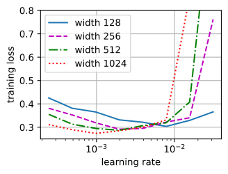
width  128: best lr 7.8e-03
width  256: best lr 3.9e-03
width  512: best lr 2.0e-03
width 1024: best lr 9.8e-04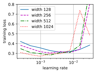
Each width traces a U: too small a learning rate undertrains, too large destabilizes — the widest curves climb off the top of the chart on the right, where the capped runs sit. But the U’s do not line up. The minimum slides steadily left as the network widens: in these runs the best learning rate at width 1,024 is about eight times smaller than at width 128, and the drift continues at larger widths (Yang et al. 2022). Two observations follow from these fixed-seed runs. First, after tuning, the wider models match or improve on the narrower models’ training loss. Second, the preferred regions do not transfer: the width-128 optimum places the width-1,024 model on the unstable branch of its curve, and the converse undertrains the narrower model. Under standard parametrization, the selected learning rate therefore depends on width as well as on the task.
9.11.1.3 Why It Moves
The first-step activation change explains the drift and determines the layerwise correction. Consider a hidden weight matrix \(\mathbf{W} \in \mathbb{R}^{n \times n}\) receiving activations \(\mathbf{h}\) with entries of typical size \(\overline{|h|}\). For a single example its gradient is an outer product, \(\mathbf{g} = \boldsymbol{\delta} \mathbf{h}^\top\), where \(\boldsymbol{\delta}\) is the backpropagated error. On the very first step Adam’s ratio \(\hat{\mathbf{m}}/\sqrt{\hat{\mathbf{v}}}\) equals \(\operatorname{sign}(\mathbf{g})\) exactly, the sign-descent connection of Section 9.6 with no smoothing yet. The sign of an outer product factorizes, so the update’s effect on the layer’s output is
\[ (\Delta\mathbf{W}\, \mathbf{h})_i = -\eta \sum_{j=1}^{n} \operatorname{sign}(\delta_i h_j)\, h_j = -\eta\, \operatorname{sign}(\delta_i) \sum_{j=1}^{n} |h_j| \approx -\eta\, n\, \overline{|h|}. \tag{9.11.1}\]
For this single-example first step, all \(n\) terms add coherently because the update is correlated with the incoming activations. The resulting change in each output coordinate is therefore about \(\eta n \overline{|h|}\). (A minibatch gradient is a sum of such outer products and its sign does not factorize, so read this as the leading-order intuition; the coordinate check below confirms the width scaling empirically.) In this approximation, doubling the width doubles the activation change, so the largest stable \(\eta\) scales inversely with width; the sweep shows a similar trend in the preferred learning rate. The effect is also per layer: the input layer’s fan-in is 784 at every width, and biases have no fan-in at all, so their stable learning rates do not move. A single global \(\eta\) is a compromise between layers that scale differently, and it is the hidden matrices that drag it down.
9.11.2 Maximal Update Parametrization
9.11.2.1 The Rules
If each layer’s stable learning rate scales differently with width, then a single learning rate should not be asked to serve them all. The maximal update parametrization (Yang et al. 2022) encodes the width dependence through per-component scaling rules: relative to a chosen base width, each layer’s learning rate (and one forward-pass scale factor) absorbs its own scaling, and what remains is the base learning rate, which is width-independent and can be tuned on the smallest member of the family. The scaling is not guessed; it is derived from the infinite-width limit in which every layer’s activations remain of order one and every layer keeps learning features (Yang and Hu 2021). Larger update scales cause activations to grow with width, as in Equation 9.11.1; smaller asymptotic scales suppress feature learning. “Maximal update” denotes the largest width scaling that preserves stable activations and nontrivial feature updates in the infinite-width analysis.
For Adam-family optimizers and a width multiplier \(m = n / n_{\text{base}}\), the rules are compact.
:The maximal update parametrization for Adam, relative to a chosen base width. The hidden-matrix learning rate and output-logit multiplier depend on width; the listed initialization scales, input and bias learning rates, and other forward operations remain unchanged.
| parameters | initialization | Adam learning rate | forward pass |
|---|---|---|---|
| input weights and all biases | unchanged | \(\eta\) | unchanged |
| hidden matrices | variance \(\propto 1/\text{fan-in}\) (unchanged) | \(\eta / m\) | unchanged |
| output matrix | unchanged | \(\eta\) | logits \(\times\, 1/m\) |
The initialization column is the one thing that does not change: variance \(\propto 1/\text{fan-in}\) is correct at every width, and we already wrote it into MLP. The hidden learning rate shrinks as \(1/m\), cancelling the \(n\)-fold coherence of Equation 9.11.1. The output layer keeps its learning rate but its logits are divided by \(m\), which tames the same coherence on the output side while letting the head keep learning. Input weights and biases, whose fan-in never grows, are left alone — for language models the token embedding falls in this class too, which is why muP treats embeddings apart from hidden matrices. Transformers need one further rule (attention logits scaled by \(1/d\) rather than \(1/\sqrt{d}\)), SGD has its own column of exponents, and several algebraically equivalent formulations circulate; the practitioner’s guide by Dey et al. (2024) lays out the full table and the pitfalls. Here the whole change is a subclass:
class MuMLP(MLP):
    """The same network under muP, relative to a width-128 base."""
    def __init__(self, width, base_width=128):
        super().__init__(width)
        self.m = width / base_width

    def forward(self, X):
        # rule 1: scale the output matrix's logits; the bias is untouched
        return self.fc_out(self.features(X) / self.m)

    def configure_adam(self, lr):
        hidden = [self.fc_h1.weight, self.fc_h2.weight]
        rest = [p for p in self.parameters()
                if not any(p is q for q in hidden)]
        return torch.optim.Adam([              # rule 2: hidden LR / m
            {'params': rest, 'lr': lr},
            {'params': hidden, 'lr': lr / self.m}])
class MuMLP(MLP):
"""The same network under muP, relative to a width-128 base."""
def __init__(self, width, base_width=128, rngs=None):
super().__init__(width, rngs=rngs)
self.m = width / base_width
def __call__(self, X):
# rule 1: scale the output matrix's logits; the bias is untouched
return self.fc_out(self.features(X) / self.m)
def configure_adam(self, lr):
def labels(params): # rule 2: hidden LR / m
return jax.tree_util.tree_map_with_path(
lambda path, _: 'hidden'
if 'fc_h' in jax.tree_util.keystr(path)
and 'kernel' in jax.tree_util.keystr(path) else 'rest',
params)
tx = optax.multi_transform(
{'hidden': optax.adam(lr / self.m), 'rest': optax.adam(lr)},
labels)
return nnx.Optimizer(self, tx, wrt=nnx.Param)At the base width, \(m = 1\) and MuMLP is MLP exactly — muP changes nothing about the model you tune, only about how its siblings scale.
9.11.2.2 The Coordinate Check
A coordinate check is a low-cost diagnostic for a muP implementation and is recommended by the practitioner’s guide (Dey et al. 2024). The coordinate check tests the width scaling predicted by Equation 9.11.1. Under the rules used here, hidden activations should remain of order one after a training step, while the output logits follow their explicit \(1/m\) scaling. Unintended activation growth with width indicates a scaling error. So we instantiate the family across widths, apply one Adam update at a mid-grid learning rate, and record the mean absolute activation of each layer. One step is the cleanest probe — Equation 9.11.1 is exact there, while further steps compound the growth but entangle it with feedback from the loss.
def activations(model, Xb):
    with torch.no_grad():
        h1 = F.relu(model.fc_in(Xb))
        h2 = F.relu(model.fc_h1(h1))
        h3 = F.relu(model.fc_h2(h2))
        return [float(h.abs().mean()) for h in (h1, h2, h3, model(Xb))]

def coord_check(arch, widths, lr=2**-8, num_steps=1):
    Xb, Yb = X[:256], Y[:256]
    sizes = []
    for width in widths:
        torch.manual_seed(0)
        model = arch(width).to(device)
        optimizer = model.configure_adam(lr)
        for _ in range(num_steps):
            train_step(model, optimizer, Xb, Yb)
        sizes.append(activations(model, Xb))
    return list(zip(*sizes))
def activations(model, Xb):
h1 = nnx.relu(model.fc_in(Xb))
h2 = nnx.relu(model.fc_h1(h1))
h3 = nnx.relu(model.fc_h2(h2))
return [float(jnp.abs(h).mean()) for h in (h1, h2, h3, model(Xb))]
def coord_check(arch, widths, lr=2**-8, num_steps=1):
Xb, Yb = X[:256], Y[:256]
sizes = []
for width in widths:
model = arch(width, rngs=nnx.Rngs(0))
optimizer = model.configure_adam(lr)
for _ in range(num_steps):
train_step(model, optimizer, Xb, Yb)
sizes.append(activations(model, Xb))
return list(zip(*sizes))First under standard parametrization. We extend the width range to 4,096 — the check costs seconds, allowing evaluation beyond the widths used in the training sweep:
check_widths = [128, 256, 512, 1024, 2048, 4096]
sp_acts = coord_check(MLP, check_widths)
d2l.plot(check_widths, list(sp_acts), 'width', 'mean |activation|',
         xscale='log', yscale='log',
         legend=['layer 1', 'layer 2', 'layer 3', 'logits'])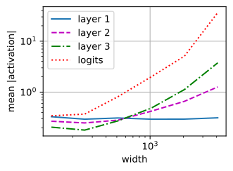
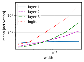
The plot is Equation 9.11.1 made visible. Layer 1, which sits behind the fixed-fan-in input matrix, is flat. Layers 2 and 3, behind the square matrices, grow with width — and the growth compounds with depth, each layer feeding its excess to the next, so the logits grow by roughly two orders of magnitude across this range. This growth explains why a first-step learning rate that is stable at narrow widths can destabilize a sufficiently wide model. We next repeat the check under muP:
mup_acts = coord_check(MuMLP, check_widths)
d2l.plot(check_widths, list(mup_acts), 'width', 'mean |activation|',
         xscale='log', yscale='log',
         legend=['layer 1', 'layer 2', 'layer 3', 'logits'])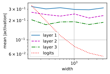
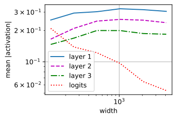
All three layer curves are flat: no layer’s update scale depends on width anymore. The logits curve falls with width rather than staying level, and this is by design — the \(1/m\) output multiplier starts the logits small, and they grow to order one through learning (the coherent alignment of Equation 9.11.1, now correctly budgeted) rather than through size. Growth is the unambiguous failure; flat or falling says only that the forward pass is stable, since the check reads activation sizes, not feature learning — updates shrinking too fast would also read as falling, with the layer quietly frozen. This one-figure test can reveal common muP implementation errors, including a missing multiplier, a mislabeled layer, or an unintentionally restored framework default. The exercises introduce these errors and use the coordinate check to detect them.
9.11.2.3 Learning-Rate Transfer
The coordinate check tests activation scaling. We next repeat the learning-rate sweep under muP to test transfer:
mup_loss = {w: [train_mlp(MuMLP, w, lr) for lr in lrs] for w in widths}
for w in widths:
    print(f'width {w:4d}: best lr {min(zip(mup_loss[w], lrs))[1]:.1e}')
d2l.plot(lrs, [mup_loss[w] for w in widths], 'learning rate',
         'training loss', xscale='log', ylim=[0.25, 0.8],
legend=[f'width {w}' for w in widths])width 128: best lr 7.8e-03
width 256: best lr 7.8e-03
width 512: best lr 7.8e-03
width 1024: best lr 7.8e-03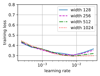
width  128: best lr 7.8e-03
width  256: best lr 7.8e-03
width  512: best lr 7.8e-03
width 1024: best lr 7.8e-03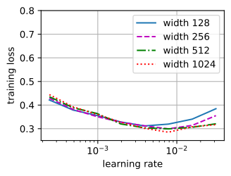
The width-128 curve is identical to before, as it must be. For the other three widths, the preferred region no longer shows the systematic leftward movement seen under standard parametrization. Across the eightfold width change, each grid minimum lies within one or two steps of the base-width minimum. With the base width’s selected learning rate reused at width 1,024, the muP run finishes within a few percent of that width’s lowest loss in the grid; the standard-parametrization run is 15–20% above its grid minimum. Because each point is a single seeded run, these values describe this experiment rather than population uncertainty. This is hyperparameter transfer: tune the base model, scale up, keep the numbers. Two caveats belong next to the result. On this small family, retuning the wide model directly costs nothing, and standard parametrization retuned at width 1,024 reaches a comparable loss — muP’s value is not a better optimum but not needing the sweep at the width where sweeps are unaffordable. And transfer is a statement about the base learning rate, not a warranty on every knob: schedules, batch size, and regularization still interact with scale (Section 9.10). A published large-scale application reports the same transfer procedure: Yang et al. (2022) tuned a 6.7-billion-parameter GPT-3 by sweeping a 40-million-parameter proxy, spending about 7% of the pretraining budget on tuning and outperforming the original model.
9.11.3 The Spectral View
muP arrived through infinite-width limits, but there is a shorter road that connects it to Section 9.9. There we measured an update by the right norm for a matrix acting between spaces of different sizes; the healthy scale for a layer mapping \(n_{\text{in}}\) activations to \(n_{\text{out}}\) is spectral norm on the order of \(\sqrt{n_{\text{out}} / n_{\text{in}}}\), for weights and updates alike:
\[ \|\mathbf{W}\|_2 \asymp \sqrt{\frac{n_{\text{out}}}{n_{\text{in}}}}, \qquad \|\Delta\mathbf{W}\|_2 \asymp \sqrt{\frac{n_{\text{out}}}{n_{\text{in}}}}. \tag{9.11.2}\]
Yang et al. (2023) show that this spectral condition is equivalent to muP: the per-layer learning rates and multipliers of Table 9.11.1 are exactly what it takes to make Adam’s raw updates land at the right spectral scale at every width, since otherwise their spectral norm grows with the layer’s dimensions, as Equation 9.11.1 witnessed. Seen this way, muP can be viewed as per-layer scaling that converts Adam’s coordinatewise updates to the desired spectral scale. An optimizer whose matrix update rule directly controls that scale may require fewer external adjustments: Muon orthogonalizes each hidden matrix’s update and scales it per shape (Jordan et al. 2024; Bernstein and Newhouse 2024), so much of muP’s per-layer control comes built in — though its RMS-matched scale is an empirical convention, not the \(\sqrt{n_{\text{out}} / n_{\text{in}}}\) of Equation 9.11.2, a distinction Section 9.9 already flagged. This is one reason learning rates chosen for Muon-family optimizers tend to change less with width.
9.11.4 Hyperparameter Transfer in Large Runs
Proxy-model tuning and transfer are common in large-scale training, but the mechanism varies. Cerebras adopted muP directly: the Cerebras-GPT family was trained with hyperparameters transferred from a roughly 40-million-parameter proxy, with the coordinate check as part of the release (Dey et al. 2023). DeepSeek took the empirical road instead: rather than removing the drift, they measured it, fitting power laws for the optimal learning rate and batch size as functions of the compute budget across many small runs and extrapolating the fit to the target scale (DeepSeek-AI et al. 2024). Meta reports training Llama 4 with an in-house scheme called MetaP for setting per-layer learning rates and initialization scales that transfer across width, depth, batch size, and token budget — with methodology undisclosed (Meta AI 2025). And Moonshot used no width-dependent parametrization at all when training Kimi K2 with Muon over 15.5 trillion tokens: they scale every layer’s update to a fixed root-mean-square size matched empirically to AdamW’s typical update (Liu et al. 2025; Kimi Team 2025) — per-layer control done by measurement inside the optimizer, the spectral view’s conclusion reached by engineering rather than by limit theorems.
The theory itself is still moving. Kosson et al. (2025) present evidence that muP’s assumptions describe only the first stretch of training: in long runs with weight decay, update dynamics equilibrate to a width-independent regime on their own, weight decay rather than parametrization does the stabilizing, and muP’s contribution resembles an implicit warmup that a schedule could replace. Whether that account or the spectral one better explains transfer in practice is an open question. The practical reading for now: transfer is the shared goal, muP is one working mechanism for it rather than settled law, and the coordinate check is worth running on any model family you intend to scale, whatever parametrization you choose. It is inexpensive and provides a direct check of the expected width-dependent activation pattern.
9.11.5 Summary
Hyperparameters tuned on a small model do not transfer by default: the best learning rate drifts down as the network widens, because one Adam step perturbs a hidden layer’s activations in proportion to its fan-in (Equation 9.11.1). The maximal update parametrization removes the width dependence with per-layer rules: initialization variance \(\propto 1/\text{fan-in}\) as usual, hidden-matrix learning rates scaled by \(1/m\), logits scaled by \(1/m\), inputs and biases left alone. In this model family, the preferred learning-rate region then remains close to the base-width selection across the tested widths. The coordinate check evaluates such a scheme in seconds: activation scales should follow the parametrization’s prescribed width dependence without unintended growth after a training step. Spectrally, muP makes Adam’s updates land at the norm scale a layer’s shape prescribes, much of which Muon-style optimizers build in through their own shape-scaled updates. Production practice spans principled parametrization, fitted scaling laws, and empirically matched update sizes; the goal of transfer is common to all of them.
9.11.6 Exercises
- Our coordinate check varies width at fixed depth. Generalize
MLPfrom its three hidden layers to \(L\) of them and run the check across \(L \in \{3, 6, 12, 24\}\) at fixed width, under both parametrizations. Does muP’s width scaling keep activations flat across depth? What does that tell you about what muP does and does not promise? - Verify transfer directly: under each parametrization, find the best learning rate at width 256 by sweeping, apply it unchanged at width 1,024, and compare the loss against the best learning rate found by sweeping at width 1,024. Report all four optima.
- Break muP on purpose: delete the \(1/m\) logit scaling from
MuMLPbut keep the hidden learning-rate rule, and rerun the coordinate check. Which curve catches the bug? Repeat, this time keeping the multiplier but giving the hidden matrices the full learning rate. - Replace Adam with weight-decayed AdamW (Section 9.7) in the standard-parametrization sweep and train several times longer. Does the optimum drift less? Relate what you see to the argument of Kosson et al. (2025) that weight decay, not parametrization, stabilizes long runs.