from d2l import torch as d2l
import torch
from torch import nn
from torch.nn import functional as F6.2 Convolutions for Images
The preceding section derived convolutional layers from locality and translation equivariance. We now define the two-dimensional cross-correlation operation, implement it directly, and show how its kernels can be learned from image data.
from d2l import tensorflow as d2l
import tensorflow as tf
from d2l import jax as d2l
from flax import nnx
import jax
from jax import numpy as jnpfrom d2l import mxnet as d2l
from mxnet import autograd, gluon, np, npx
from mxnet.gluon import nn
npx.set_np()6.2.1 The Cross-Correlation Operation
Strictly speaking, the operation used by a convolutional layer is cross-correlation rather than mathematical convolution. As described in Section 6.1, such a layer combines an input tensor and a kernel tensor into an output tensor through a cross-correlation operation.
We first omit channels and consider two-dimensional inputs and hidden representations. In Figure 6.2.1, the input is a two-dimensional tensor with a height of 3 and width of 3. We mark the shape of the tensor as \(3 \times 3\) or (\(3\), \(3\)). The height and width of the kernel are both 2. The shape of the kernel window (or convolution window) is given by the height and width of the kernel (here it is \(2 \times 2\)).
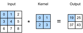
In the two-dimensional cross-correlation operation, we begin with the convolution window positioned at the upper-left corner of the input tensor and slide it across the input tensor, both from left to right and top to bottom. When the convolution window slides to a certain position, the input subtensor contained in that window and the kernel tensor are multiplied elementwise and the resulting tensor is summed up yielding a single scalar value. This result gives the value of the output tensor at the corresponding location. Here, the output tensor has a height of 2 and width of 2 and the four elements are derived from the two-dimensional cross-correlation operation:
\[ \begin{aligned} 0\times0+1\times1+3\times2+4\times3 &= 19,\\ 1\times0+2\times1+4\times2+5\times3 &= 25,\\ 3\times0+4\times1+6\times2+7\times3 &= 37,\\ 4\times0+5\times1+7\times2+8\times3 &= 43. \end{aligned} \]
Along each axis, the output is smaller than the input. Because the kernel has width and height greater than \(1\), we can only properly compute the cross-correlation for locations where the kernel fits wholly within the image. The output size is therefore the input size \(n_\textrm{h} \times n_\textrm{w}\) minus the size of the convolution kernel \(k_\textrm{h} \times k_\textrm{w}\), that is,
\[(n_\textrm{h}-k_\textrm{h}+1) \times (n_\textrm{w}-k_\textrm{w}+1). \tag{6.2.1}\]
The kernel must fit within the image at every evaluated position. The next section shows how to keep the size unchanged by padding the image with zeros around its boundary so that there is enough space to shift the kernel. Next, we implement this process in the corr2d function, which accepts an input tensor X and a kernel tensor K and returns an output tensor Y.
def corr2d(X, K):
    """Compute 2D cross-correlation."""
    h, w = K.shape
    Y = d2l.zeros((X.shape[0] - h + 1, X.shape[1] - w + 1))
    for i in range(Y.shape[0]):
        for j in range(Y.shape[1]):
            Y[i, j] = d2l.reduce_sum((X[i: i + h, j: j + w] * K))
    return Y
def corr2d(X, K):
"""Compute 2D cross-correlation."""
h, w = K.shape
Y = tf.Variable(tf.zeros((X.shape[0] - h + 1, X.shape[1] - w + 1)))
for i in range(Y.shape[0]):
for j in range(Y.shape[1]):
Y[i, j].assign(tf.reduce_sum(
X[i: i + h, j: j + w] * K))
return Ydef corr2d(X, K):
"""Compute 2D cross-correlation."""
h, w = K.shape
Y = jnp.zeros((X.shape[0] - h + 1, X.shape[1] - w + 1))
for i in range(Y.shape[0]):
for j in range(Y.shape[1]):
Y = Y.at[i, j].set((X[i:i + h, j:j + w] * K).sum())
return Ydef corr2d(X, K):
"""Compute 2D cross-correlation."""
h, w = K.shape
Y = d2l.zeros((X.shape[0] - h + 1, X.shape[1] - w + 1))
for i in range(Y.shape[0]):
for j in range(Y.shape[1]):
Y[i, j] = d2l.reduce_sum((X[i: i + h, j: j + w] * K))
return YWe can construct the input tensor X and the kernel tensor K from Figure 6.2.1 to validate the output of the above implementation of the two-dimensional cross-correlation operation.
X = d2l.tensor([[0.0, 1.0, 2.0], [3.0, 4.0, 5.0], [6.0, 7.0, 8.0]])
K = d2l.tensor([[0.0, 1.0], [2.0, 3.0]])
corr2d(X, K)tensor([[19., 25.],
[37., 43.]])<tf.Variable 'Variable:0' shape=(2, 2) dtype=float32, numpy=
array([[19., 25.],
[37., 43.]], dtype=float32)>Array([[19., 25.],
[37., 43.]], dtype=float32)array([[19., 25.],
[37., 43.]])6.2.2 Convolutional Layers
A convolutional layer cross-correlates the input and kernel and adds a scalar bias to produce an output. The two parameters of a convolutional layer are the kernel and the scalar bias. When training models based on convolutional layers, we typically initialize the kernels randomly, as with a fully connected layer.
We are now ready to implement a two-dimensional convolutional layer based on the corr2d function defined above. In the __init__ constructor method, we declare weight and bias as the two model parameters. The forward propagation method calls the corr2d function and adds the bias.
class Conv2D(nn.Module):
    def __init__(self, kernel_size):
        super().__init__()
        self.weight = nn.Parameter(torch.rand(kernel_size))
        self.bias = nn.Parameter(torch.zeros(1))

    def forward(self, x):
        return corr2d(x, self.weight) + self.bias
class Conv2D(tf.keras.layers.Layer):
def __init__(self):
super().__init__()
def build(self, kernel_size):
initializer = tf.random_normal_initializer()
self.weight = self.add_weight(name='w', shape=kernel_size,
initializer=initializer)
self.bias = self.add_weight(name='b', shape=(1, ),
initializer=initializer)
def call(self, inputs):
return corr2d(inputs, self.weight) + self.biasclass Conv2D(nnx.Module):
def __init__(self, kernel_size, rngs=None):
rngs = nnx.Rngs(d2l.get_key()) if rngs is None else rngs
self.weight = nnx.Param(
nnx.initializers.uniform()(rngs.params(), kernel_size))
self.bias = nnx.Param(jnp.zeros(1))
def __call__(self, x):
return corr2d(x, self.weight) + self.biasclass Conv2D(nn.Block):
def __init__(self, kernel_size):
super().__init__()
self.weight = gluon.Parameter('weight', shape=kernel_size)
self.bias = gluon.Parameter('bias', shape=(1,))
def forward(self, x):
return corr2d(x, self.weight.data()) + self.bias.data()In an \(h \times w\) convolution, or an \(h \times w\) convolution kernel, the height and width of the kernel are \(h\) and \(w\), respectively. We call a convolutional layer with this kernel an \(h \times w\) convolutional layer.
6.2.3 Object Edge Detection in Images
As a first application, we use a convolutional layer to detect an object’s edge by locating changes in pixel values. First, we construct an “image” of \(6\times 8\) pixels. The middle four columns are black (\(0\)) and the rest are white (\(1\)).
X = d2l.ones((6, 8))
X[:, 2:6] = 0
X
tensor([[1., 1., 0., 0., 0., 0., 1., 1.],
[1., 1., 0., 0., 0., 0., 1., 1.],
[1., 1., 0., 0., 0., 0., 1., 1.],
[1., 1., 0., 0., 0., 0., 1., 1.],
[1., 1., 0., 0., 0., 0., 1., 1.],
[1., 1., 0., 0., 0., 0., 1., 1.]])X = tf.Variable(tf.ones((6, 8)))
X[:, 2:6].assign(tf.zeros(X[:, 2:6].shape))
X<tf.Variable 'Variable:0' shape=(6, 8) dtype=float32, numpy=
array([[1., 1., 0., 0., 0., 0., 1., 1.],
[1., 1., 0., 0., 0., 0., 1., 1.],
[1., 1., 0., 0., 0., 0., 1., 1.],
[1., 1., 0., 0., 0., 0., 1., 1.],
[1., 1., 0., 0., 0., 0., 1., 1.],
[1., 1., 0., 0., 0., 0., 1., 1.]], dtype=float32)>X = jnp.ones((6, 8))
X = X.at[:, 2:6].set(0)
XArray([[1., 1., 0., 0., 0., 0., 1., 1.],
[1., 1., 0., 0., 0., 0., 1., 1.],
[1., 1., 0., 0., 0., 0., 1., 1.],
[1., 1., 0., 0., 0., 0., 1., 1.],
[1., 1., 0., 0., 0., 0., 1., 1.],
[1., 1., 0., 0., 0., 0., 1., 1.]], dtype=float32)X = d2l.ones((6, 8))
X[:, 2:6] = 0
Xarray([[1., 1., 0., 0., 0., 0., 1., 1.],
[1., 1., 0., 0., 0., 0., 1., 1.],
[1., 1., 0., 0., 0., 0., 1., 1.],
[1., 1., 0., 0., 0., 0., 1., 1.],
[1., 1., 0., 0., 0., 0., 1., 1.],
[1., 1., 0., 0., 0., 0., 1., 1.]])Next, we construct a kernel K with a height of 1 and a width of 2. When we perform the cross-correlation operation with the input, if the horizontally adjacent elements are the same, the output is 0. Otherwise, the output is nonzero. This kernel is a special case of a finite-difference operator. At location \((i,j)\) it computes \(x_{i,j} - x_{i,j+1}\), the difference between horizontally adjacent pixels. Up to a sign, this is a discrete approximation to the first derivative in the horizontal direction. For a function \(f(i,j)\), the derivative is
\[\partial_j f(i,j) = \lim_{\epsilon \to 0} \frac{f(i,j+\epsilon) - f(i,j)}{\epsilon}, \tag{6.2.2}\]
so the kernel output \(x_{i,j} - x_{i,j+1}\) approximates \(-\partial_j f(i,j)\).
K = d2l.tensor([[1.0, -1.0]])We are ready to perform the cross-correlation operation with arguments X (our input) and K (our kernel). The output is \(1\) at the edge from white to black and \(-1\) for the edge from black to white. All other outputs take value \(0\).
Y = corr2d(X, K)
Ytensor([[ 0., 1., 0., 0., 0., -1., 0.],
[ 0., 1., 0., 0., 0., -1., 0.],
[ 0., 1., 0., 0., 0., -1., 0.],
[ 0., 1., 0., 0., 0., -1., 0.],
[ 0., 1., 0., 0., 0., -1., 0.],
[ 0., 1., 0., 0., 0., -1., 0.]])<tf.Variable 'Variable:0' shape=(6, 7) dtype=float32, numpy=
array([[ 0., 1., 0., 0., 0., -1., 0.],
[ 0., 1., 0., 0., 0., -1., 0.],
[ 0., 1., 0., 0., 0., -1., 0.],
[ 0., 1., 0., 0., 0., -1., 0.],
[ 0., 1., 0., 0., 0., -1., 0.],
[ 0., 1., 0., 0., 0., -1., 0.]], dtype=float32)>Array([[ 0., 1., 0., 0., 0., -1., 0.],
[ 0., 1., 0., 0., 0., -1., 0.],
[ 0., 1., 0., 0., 0., -1., 0.],
[ 0., 1., 0., 0., 0., -1., 0.],
[ 0., 1., 0., 0., 0., -1., 0.],
[ 0., 1., 0., 0., 0., -1., 0.]], dtype=float32)array([[ 0., 1., 0., 0., 0., -1., 0.],
[ 0., 1., 0., 0., 0., -1., 0.],
[ 0., 1., 0., 0., 0., -1., 0.],
[ 0., 1., 0., 0., 0., -1., 0.],
[ 0., 1., 0., 0., 0., -1., 0.],
[ 0., 1., 0., 0., 0., -1., 0.]])We can now apply the kernel to the transposed image. As expected, it vanishes. The kernel K only detects vertical edges.
corr2d(d2l.transpose(X), K)tensor([[0., 0., 0., 0., 0.],
[0., 0., 0., 0., 0.],
[0., 0., 0., 0., 0.],
[0., 0., 0., 0., 0.],
[0., 0., 0., 0., 0.],
[0., 0., 0., 0., 0.],
[0., 0., 0., 0., 0.],
[0., 0., 0., 0., 0.]])<tf.Variable 'Variable:0' shape=(8, 5) dtype=float32, numpy=
array([[0., 0., 0., 0., 0.],
[0., 0., 0., 0., 0.],
[0., 0., 0., 0., 0.],
[0., 0., 0., 0., 0.],
[0., 0., 0., 0., 0.],
[0., 0., 0., 0., 0.],
[0., 0., 0., 0., 0.],
[0., 0., 0., 0., 0.]], dtype=float32)>Array([[0., 0., 0., 0., 0.],
[0., 0., 0., 0., 0.],
[0., 0., 0., 0., 0.],
[0., 0., 0., 0., 0.],
[0., 0., 0., 0., 0.],
[0., 0., 0., 0., 0.],
[0., 0., 0., 0., 0.],
[0., 0., 0., 0., 0.]], dtype=float32)array([[0., 0., 0., 0., 0.],
[0., 0., 0., 0., 0.],
[0., 0., 0., 0., 0.],
[0., 0., 0., 0., 0.],
[0., 0., 0., 0., 0.],
[0., 0., 0., 0., 0.],
[0., 0., 0., 0., 0.],
[0., 0., 0., 0., 0.]])6.2.4 Learning a Kernel
The finite difference [1, -1] works when the desired feature is known in advance. For larger kernels and successive convolutional layers, manually specifying every filter is generally impractical.
We therefore learn the kernel that maps X to Y from input–output pairs. We first construct a convolutional layer and initialize its kernel as a random tensor. Next, in each iteration, we will use the squared error to compare Y with the output of the convolutional layer. We can then calculate the gradient to update the kernel. The following example uses the built-in two-dimensional convolutional layer and omits the bias.
# Construct a two-dimensional convolutional layer with 1 output channel and a
# kernel of shape (1, 2). For the sake of simplicity, we ignore the bias here
conv2d = nn.LazyConv2d(1, kernel_size=(1, 2), bias=False)

# The two-dimensional convolutional layer uses four-dimensional input and
# output in the format of (example, channel, height, width), where the batch
# size (number of examples in the batch) and the number of channels are both 1
X = X.reshape((1, 1, 6, 8))
Y = Y.reshape((1, 1, 6, 7))
lr = 3e-2  # Learning rate

for i in range(10):
    Y_hat = conv2d(X)
    l = (Y_hat - Y) ** 2
    conv2d.zero_grad()
    l.sum().backward()
    # Update the kernel
    with torch.no_grad():
        conv2d.weight[:] -= lr * conv2d.weight.grad
    if (i + 1) % 2 == 0:
        print(f'epoch {i + 1}, loss {l.sum():.3f}')
epoch 2, loss 9.572
epoch 4, loss 2.071
epoch 6, loss 0.538
epoch 8, loss 0.168
epoch 10, loss 0.060# Construct a two-dimensional convolutional layer with 1 output channel and a
# kernel of shape (1, 2). For the sake of simplicity, we ignore the bias here
conv2d = tf.keras.layers.Conv2D(1, (1, 2), use_bias=False)
# The two-dimensional convolutional layer uses four-dimensional input and
# output in the format of (example, height, width, channel), where the batch
# size (number of examples in the batch) and the number of channels are both 1
X = tf.reshape(X, (1, 6, 8, 1))
Y = tf.reshape(Y, (1, 6, 7, 1))
lr = 3e-2 # Learning rate
for i in range(10):
with tf.GradientTape() as g:
Y_hat = conv2d(X)
l = (Y_hat - Y) ** 2
# Update the kernel
update = tf.multiply(lr, g.gradient(l, conv2d.trainable_weights)[0])
conv2d.kernel.assign(conv2d.kernel - update)
if (i + 1) % 2 == 0:
print(f'epoch {i + 1}, loss {tf.reduce_sum(l):.3f}')epoch 2, loss 28.971
epoch 4, loss 10.855
epoch 6, loss 4.276
epoch 8, loss 1.723
epoch 10, loss 0.701# Construct a two-dimensional convolutional layer with 1 output channel and a
# kernel of shape (1, 2). For the sake of simplicity, we ignore the bias here.
# Use a small-stddev normal init so the toy 10-step SGD has time to converge
# (Flax's default lecun_normal yields a much larger initial loss).
conv2d = nnx.Conv(1, 1, kernel_size=(1, 2), use_bias=False, padding='VALID',
kernel_init=nnx.initializers.normal(stddev=0.01),
rngs=nnx.Rngs(d2l.get_key()))
# The two-dimensional convolutional layer uses four-dimensional input and
# output in the format of (example, height, width, channel), where the batch
# size (number of examples in the batch) and the number of channels are both 1
X = X.reshape((1, 6, 8, 1))
Y = Y.reshape((1, 6, 7, 1))
lr = 3e-2 # Learning rate
def loss(model, X, Y):
Y_hat = model(X)
return ((Y_hat - Y) ** 2).sum()
for i in range(10):
l, grads = nnx.value_and_grad(loss)(conv2d, X, Y)
conv2d.kernel[...] -= lr * grads.kernel[...]
if (i + 1) % 2 == 0:
print(f'epoch {i + 1}, loss {l:.3f}')epoch 2, loss 4.868
epoch 4, loss 0.817
epoch 6, loss 0.137
epoch 8, loss 0.023
epoch 10, loss 0.004# Construct a two-dimensional convolutional layer with 1 output channel and a
# kernel of shape (1, 2). For the sake of simplicity, we ignore the bias here
conv2d = nn.Conv2D(1, kernel_size=(1, 2), use_bias=False)
conv2d.initialize()
# The two-dimensional convolutional layer uses four-dimensional input and
# output in the format of (example, channel, height, width), where the batch
# size (number of examples in the batch) and the number of channels are both 1
X = X.reshape(1, 1, 6, 8)
Y = Y.reshape(1, 1, 6, 7)
lr = 3e-2 # Learning rate
for i in range(10):
with autograd.record():
Y_hat = conv2d(X)
l = (Y_hat - Y) ** 2
l.backward()
# Update the kernel
conv2d.weight.data()[:] -= lr * conv2d.weight.grad()
if (i + 1) % 2 == 0:
print(f'epoch {i + 1}, loss {float(l.sum()):.3f}')epoch 2, loss 5.154
epoch 4, loss 0.865
epoch 6, loss 0.145
epoch 8, loss 0.024
epoch 10, loss 0.004After 10 iterations, the error is small. We can inspect the learned kernel.
d2l.reshape(conv2d.weight.data, (1, 2))tensor([[ 1.0096, -0.9616]])d2l.reshape(conv2d.get_weights()[0], (1, 2))<tf.Tensor: shape=(1, 2), dtype=float32, numpy=array([[ 1.0756308, -0.903096 ]], dtype=float32)>conv2d.kernel[...].reshape((1, 2))Array([[ 0.98822 , -0.98883337]], dtype=float32)d2l.reshape(conv2d.weight.data(), (1, 2))array([[ 0.9888173, -0.9875731]])Indeed, the learned kernel tensor is close to the kernel tensor K we defined earlier.
6.2.5 Cross-Correlation and Convolution
Recall our observation from Section 6.1 of the correspondence between the cross-correlation and convolution operations. For two-dimensional layers, strict convolution as defined in Equation 6.1.6 differs from cross-correlation only by flipping the kernel horizontally and vertically before applying cross-correlation.
Since kernels are learned from data in deep learning, the outputs of convolutional layers remain unaffected whether the layers perform strict convolution or cross-correlation.
To illustrate this, suppose that a convolutional layer performs cross-correlation and learns the kernel in Figure 6.2.1, which is here denoted as the matrix \(\mathbf{K}\). Assuming that other conditions remain unchanged, when this layer instead performs strict convolution, the learned kernel \(\mathbf{K}'\) will be the same as \(\mathbf{K}\) after \(\mathbf{K}'\) is flipped both horizontally and vertically. Thus, when the convolutional layer performs strict convolution on the input in Figure 6.2.1 with \(\mathbf{K}'\), it produces the same output as in Figure 6.2.1 (the cross-correlation of the input and \(\mathbf{K}\)).
In keeping with standard terminology in deep learning literature, we will continue to refer to the cross-correlation operation as a convolution even though the operations differ mathematically. We use the term element to refer to an entry (or component) of any tensor representing a layer representation or a convolution kernel.
6.2.6 Convolution as Matrix Multiplication
Every output element in Figure 6.2.1 is a dot product: the kernel, flattened into a vector of length \(k_\textrm{h} k_\textrm{w}\), multiplied with the input patch under the window, flattened the same way. For an input of spatial size \(h \times w\), the number of such patches depends on the kernel, padding, and stride. If we extract each patch the sliding window visits, flatten it into a row, and stack the rows, we obtain a matrix with one row per output position. The entire cross-correlation then collapses into a single product of this patch matrix with the flattened kernel. The rearrangement is called im2col (it turns image patches into the columns, here rows, of a matrix).
This rewriting motivates one important family of convolution implementations. GPUs and other accelerators are built around fast dense matrix multiplication, and libraries often lower convolutions to explicit or implicit matrix products. Depending on the shapes and hardware, they may instead select direct, Winograd, FFT-based, or other specialized kernels. The explicit form costs memory: each input element is duplicated in up to \(k_\textrm{h} k_\textrm{w}\) rows. Let’s build the patch matrix for the input and kernel of Figure 6.2.1 and check that the matrix product reproduces corr2d.
X = d2l.tensor([[0.0, 1.0, 2.0], [3.0, 4.0, 5.0], [6.0, 7.0, 8.0]])
K = d2l.tensor([[0.0, 1.0], [2.0, 3.0]])
h, w = K.shape
p_h, p_w = X.shape[0] - h + 1, X.shape[1] - w + 1
patches = d2l.stack([d2l.reshape(X[i:i + h, j:j + w], (-1,))
                     for i in range(p_h) for j in range(p_w)])
Y_mat = d2l.reshape(d2l.matmul(patches, d2l.reshape(K, (-1, 1))), (p_h, p_w))
Y_mat, d2l.reduce_sum(d2l.abs(Y_mat - corr2d(X, K)))(tensor([[19., 25.],
[37., 43.]]),
tensor(0.))(<tf.Tensor: shape=(2, 2), dtype=float32, numpy=
array([[19., 25.],
[37., 43.]], dtype=float32)>,
<tf.Tensor: shape=(), dtype=float32, numpy=0.0>)(Array([[19., 25.],
[37., 43.]], dtype=float32),
Array(0., dtype=float32))(array([[19., 25.],
[37., 43.]]),
array(0.))The sum of absolute differences is zero: the one matrix product and the sliding-window loop compute the same output.
PyTorch exposes this rearrangement directly: F.unfold extracts the patch matrix (transposed, and with batch and channel dimensions), so any convolution can be written as unfold, matrix multiplication, and reshape.
X_batch = d2l.reshape(X, (1, 1, 3, 3))
patches_unfold = F.unfold(X_batch, kernel_size=(2, 2))[0].T
torch.allclose(patches_unfold, patches)TrueThe same idea also works in the opposite direction: instead of unfolding the input, we can unroll the kernel into a sparse, banded matrix that multiplies the flattened image. The exercises explore this view.
6.2.7 Feature Map and Receptive Field
As described in Section 6.1.4, the convolutional layer output in Figure 6.2.1 is sometimes called a feature map, as it can be regarded as the learned representations (features) in the spatial dimensions (e.g., width and height) that it passes on to the subsequent layer. In CNNs, for any element \(x\) of some layer, its receptive field refers to all the elements (from all the previous layers) that may affect the calculation of \(x\) during the forward propagation. The receptive field can extend beyond the valid input region when padding is used.
We use Figure 6.2.1 to illustrate the receptive field. Given the \(2 \times 2\) convolution kernel, the receptive field of the shaded output element (of value \(19\)) is the four elements in the shaded portion of the input. Now let’s denote the \(2 \times 2\) output as \(\mathbf{Y}\) and consider a deeper CNN with an additional \(2 \times 2\) convolutional layer that takes \(\mathbf{Y}\) as its input, outputting a single element \(z\). In this case, the receptive field of \(z\) on \(\mathbf{Y}\) includes all the four elements of \(\mathbf{Y}\), while the receptive field on the input includes all the nine input elements. Stacking layers therefore lets an element respond to input features over a broader area.
This layer-by-layer counting has a closed form. Consider a stack of \(L\) convolutional layers in which layer \(i\) has a \(k_i \times k_i\) kernel and stride \(s_i\) (padding affects only which outputs exist, not how far each one sees). One step at the input of layer \(i\) corresponds to \(\prod_{j=1}^{i-1} s_j\) steps at the original input, since every earlier layer with stride \(s_j\) multiplies the step size by \(s_j\). Layer \(i\)’s kernel spans \(k_i - 1\) steps of its own input, so it widens the receptive field by \((k_i - 1) \prod_{j=1}^{i-1} s_j\) input pixels. Starting from a single pixel and summing over layers, an element at the top of the stack has a receptive field of side length
\[ r = 1 + \sum_{i=1}^{L} \left( k_i - 1 \right) \prod_{j=1}^{i-1} s_j, \tag{6.2.3}\]
where the empty product for \(i = 1\) equals \(1\).
The most common case is \(L\) stacked \(3 \times 3\) layers with stride \(1\): each layer adds \(2\), so the stack sees \((2L + 1) \times (2L + 1)\) input pixels. Two such layers cover \(5 \times 5\), three cover \(7 \times 7\). This is why deep stacks of small kernels can replace single large ones: three \(3 \times 3\) layers match the receptive field of one \(7 \times 7\) layer with fewer parameters (\(27\) weights instead of \(49\) per input–output channel pair) and three nonlinearities instead of one. Strides enter through the product: after a stride-\(2\) layer (or a pooling step, Section 6.5), every later kernel counts double, so downsampling makes the receptive field grow geometrically with depth. We will use Equation 6.2.3 repeatedly when we analyze modern architectures in Chapter 7.
Equation Equation 6.2.3 gives the theoretical receptive field: the set of inputs that can affect an activation at all. Their influence is not uniform. Luo et al. (2016) measured the effective receptive field through gradients and found that it concentrates near the center of the theoretical region, with a roughly Gaussian profile in common randomly initialized and trained networks. Depth, dilation, and larger kernels enlarge the set of possible inputs; they do not guarantee that optimization will use all of it equally.
Receptive fields derive their name from neurophysiology. Experiments recording from the visual cortex of several animal species (Hubel and Wiesel 1959, 1962, 1968) found that its lower levels respond to edges and related shapes. Later, Field (1987) modeled these responses on natural images with what are, in effect, convolutional kernels. We reprint a key figure in Figure 6.2.2.
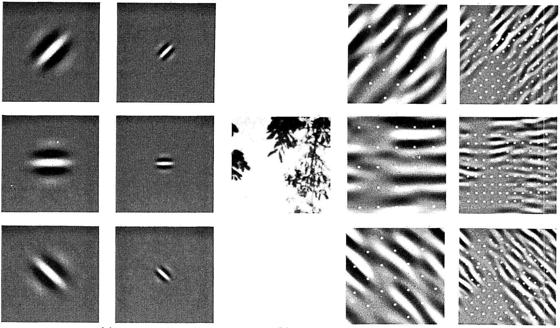
The correspondence extends to features computed by deeper layers of networks trained on image classification (Kuzovkin et al. 2018).
6.2.8 Summary
The core computation in a convolutional layer is cross-correlation. A nested loop states the operation directly; practical libraries select among implicit matrix multiplication, direct, Winograd, FFT-based, and specialized kernels. Locality creates extensive reuse of weights and overlapping input patches, but real performance depends on both arithmetic throughput and memory movement.
Convolutions can detect edges and lines, blur images, or sharpen them. In a neural network, the filters are learned from data rather than specified by hand. The language of receptive fields has a historical connection to visual neurophysiology, but that analogy is motivation rather than evidence that a particular network mirrors the brain.
6.2.9 Exercises
- Construct an image
Xwith diagonal edges.- What happens if you apply the kernel
Kin this section to it? - What happens if you transpose
X? - What happens if you transpose
K?
- What happens if you apply the kernel
- Design some kernels manually.
- Given a directional vector \(\mathbf{v} = (v_1, v_2)\), derive an edge-detection kernel that detects edges orthogonal to \(\mathbf{v}\), i.e., edges in the direction \((v_2, -v_1)\).
- Derive a finite difference operator for the second derivative. What is the minimum size of the convolutional kernel associated with it? Which structures in images respond most strongly to it?
- How would you design a blur kernel? Why might you want to use such a kernel?
- What is the minimum size of a kernel to obtain a derivative of order \(d\)?
- When you try to automatically find the gradient for the
Conv2Dclass we created, what kind of error message do you see? - How do you represent a cross-correlation operation as a matrix multiplication by changing the input and kernel tensors?