%matplotlib inline
from d2l import torch as d2l
import numpy as np
import torch9.1 Landscapes
For a deep learning problem, an optimization algorithm minimizes a specified loss function. In optimization the loss is called the objective function. By convention we minimize; maximizing a quantity is equivalent to minimizing its negative. The optimization literature also writes the parameters as a single vector \(\mathbf{x}\). For the next few sections, \(\mathbf{x}\) therefore contains all the parameters that earlier chapters wrote as \((\mathbf{w}, b)\). The main difficulty is the objective itself: a deep network’s loss is a surface over a parameter space with millions of dimensions, and its geometry determines which algorithms work. This section explains what minimizing the objective does and does not accomplish, where gradients vanish, and how curvature and noise control the progress of the methods that follow.
We describe an optimizer through three decisions. First, a descent direction specifies which way to move. The choice depends on the norm used to measure the size of a step: the negative gradient is the steepest descent direction under the Euclidean norm, and changing the norm changes the algorithm, as Section 9.9 develops. Second, a step size over time specifies how far to move along the local slope and how this distance changes during training (Section 9.8). Third, a method for controlling noise accounts for the fact that, at practical scales, the gradient is a minibatch estimate. The batch size and any averaging over time determine the variance of the update (Section 9.4, Section 9.10). Each method in this chapter, from gradient descent to Muon, is a particular way of making these three decisions.
9.1.1 The Goal of Optimization
Optimization supplies deep learning with a means, but the two have different ends. Optimization cares about the objective it was handed; learning cares about performance on data the model has never seen. As discussed in Section 2.6, training error and generalization error generally differ, and driving the first toward zero can even hurt the second. In the vocabulary of Section 2.6.1, the empirical risk is the average loss over the training set, while the risk is the expected loss over the whole population. The optimizer only ever sees the former.
%matplotlib inline
from d2l import jax as d2l
import jax
from jax import numpy as jnp
import numpy as np
For a concrete example, consider a smooth risk function \(f\) and an empirical risk function \(g\) that fluctuates around it because a finite-sample average differs from the population expectation. The minimum of the empirical risk need not sit at the minimum of the risk, and here it does not:
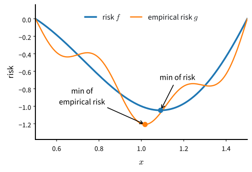
No optimizer can close this gap by itself: it arises from sampling the data, not from the optimization algorithm. Regularization and model selection address the resulting generalization problem. For the rest of the chapter we therefore set generalization aside and take the objective at face value. Even so restricted, the problem is hard. Deep learning objectives admit no analytical solution of the kind we found for linear regression in Section 2.1, so every algorithm in this chapter is iterative — and the surface it iterates over is nothing like a convex bowl.
9.1.2 Where Gradients Vanish
An iterative method needs a signal to follow, and the gradient is that signal. The classical hazards of nonconvex optimization are the places where the signal gives out: local minima, saddle points, and flat regions of saturated activations. We look at each in turn.
9.1.2.1 Local Minima
For an objective function \(f(x)\), if the value of \(f\) at \(x\) is smaller than at any nearby point, then \(x\) is a local minimum. If it is smallest over the entire domain, \(x\) is the global minimum. For example, the function
\[f(x) = x \cdot \textrm{cos}(\pi x) \textrm{ for } -1.0 \leq x \leq 2.0 \tag{9.1.1}\]
has a local minimum that is not global:
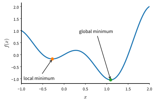
Deep learning objectives have many local minima, and an iterate that lands near one sees its gradient approach zero: from the signal alone, a local minimum is indistinguishable from the global one. Noise can dislodge the parameters, at least from a shallow basin — one reason, as we will see below, that the noise in minibatch gradients is not purely a nuisance.
9.1.2.2 Saddle Points
Besides local minima, saddle points make gradients vanish: locations where every gradient component is zero but which are neither a minimum nor a maximum of the function. Take \(f(x) = x^3\): its first and second derivatives both vanish at \(x=0\), and optimization can stall there even though it is no minimum at all. Strictly, this one-dimensional point is a stationary inflection; the true saddle geometry — down along one direction, up along another — needs at least two dimensions. Both are critical points that are not extrema, and we use “saddle” broadly for either:
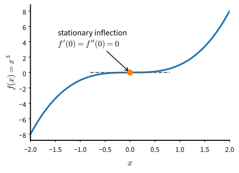
Saddle points become more prevalent in higher dimensions. Consider \(f(x, y) = x^2 - y^2\): its saddle point at \((0, 0)\) is a minimum with respect to \(x\) and a maximum with respect to \(y\), and the surface looks like the saddle that gives the phenomenon its name:
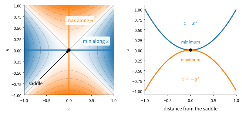
Why saddle points dominate in high dimension is a counting argument. Suppose the input of a function is a \(k\)-dimensional vector and its output a scalar, so its Hessian matrix has \(k\) eigenvalues. At a point where the gradient is zero:
- if all \(k\) eigenvalues are strictly positive — the Hessian is positive definite — we have a strict local minimum;
- if all are strictly negative, a strict local maximum;
- if some are strictly positive and some strictly negative — the Hessian is indefinite — a saddle point;
- if the nonzero eigenvalues share a sign but at least one eigenvalue is zero — the Hessian is only semidefinite, hence singular — the test is inconclusive: the flat directions are settled by higher-order terms, and the point may be a minimum, a maximum, or a saddle.
For a zero-gradient point of a high-dimensional function to be a local minimum, all of its thousands or millions of Hessian eigenvalues must be positive. If the signs were roughly balanced independent coin flips, nearly every critical point would instead be a saddle. This coin-flip argument is only a heuristic. Hessian eigenvalues at a critical point form a structured spectrum rather than independent balanced signs, as the second exercise below helps illustrate. Conditioning on criticality also relates the fraction of negative eigenvalues to the loss value. Even with these qualifications, saddles greatly outnumber exact local minima in high dimensions. Convex functions, whose Hessian eigenvalues are nowhere negative, have neither saddle points nor spurious minima. Deep learning objectives are not convex, but convex theory still supplies useful local analyses and baselines, as the final section explains.
9.1.2.3 Vanishing Gradients
The gradient can also become too small to guide an update without vanishing at a critical point. Section 4.4 explained vanishing and exploding gradients through depth and the role of initialization, while Section 8.6 analyzed the same problem through time. A one-dimensional example isolates the effect. Recall the activation functions of Section 4.1.2 and suppose we want to minimize \(f(x) = \tanh(x)\) starting from \(x = 4\). The derivative is \(f'(x) = 1 - \tanh^2(x)\), so \(f'(4) = 0.0013\): the surface is very flat at the initial point, and gradient descent barely moves for a long time before making progress.
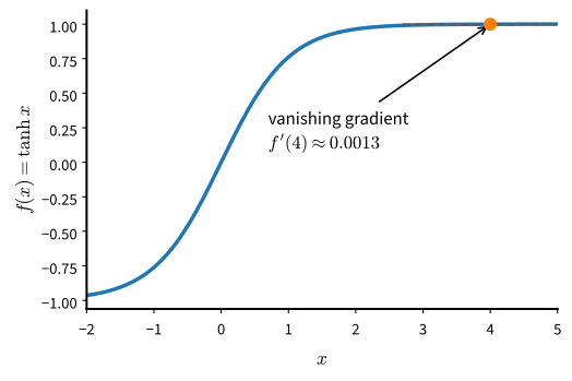
Vanishing gradients made deep networks genuinely hard to train before the ReLU activation and careful initialization; those fixes belong to model design (Section 4.1.2) rather than to the optimizer. The hazards of this section, then, are real, but two facts soften them. Deep learning does not need the global minimum — a good approximate local one serves — and, as the next section shows, what actually limits training speed day to day is usually something else.
9.1.3 Curvature and Noise
Zero-gradient points are a standard explanation for the difficulty of nonconvex optimization, but they seldom dominate routine training. Two other problems more often make training slow or unstable: curvature differs across directions, and the computed gradient is only a minibatch estimate. Most methods in this chapter address one or both of these problems.
9.1.3.1 An Ill-Conditioned Valley
Take the simplest curved objective, a quadratic valley
\[f(\mathbf{x}) = 0.1 x_1^2 + 2 x_2^2, \tag{9.1.2}\]
which curves gently along \(x_1\) (second derivative \(0.2\)) and steeply along \(x_2\) (second derivative \(4\)). Gradient descent updates both coordinates with the same learning rate \(\eta\), and each step multiplies \(x_1\) by \(1 - 0.2\,\eta\) and \(x_2\) by \(1 - 4\eta\). The steep direction sets a ceiling: for \(x_2\) to shrink rather than explode we need \(|1 - 4\eta| < 1\), that is \(\eta < 0.5\). The flat direction sets the pace: for any stable \(\eta\), each step keeps more than \(90\%\) of \(x_1\). To observe the resulting constraint, we use two helpers built in Section 9.2: d2l.train_2d iterates an update rule from a fixed starting point, and d2l.show_trace_2d draws the resulting trace over the objective’s contours. With those we run 30 steps at \(\eta = 0.45\), just under the ceiling:
def f_valley(x1, x2):  # Second derivatives 0.2 and 4
    return 0.1 * x1 ** 2 + 2 * x2 ** 2

def gd_valley(x1, x2, s1, s2):
    eta = 0.45  # Just under the stability ceiling of 0.5
    return (x1 - eta * 0.2 * x1, x2 - eta * 4 * x2, 0, 0)

d2l.show_trace_2d(f_valley, d2l.train_2d(gd_valley, steps=30))epoch 30, x1: -0.295265, x2: -0.002476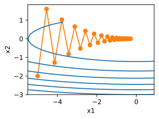
epoch 30, x1: -0.295265, x2: -0.002476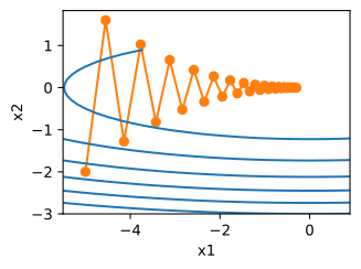
The trace shows the characteristic behavior of an ill-conditioned problem: the iterate oscillates across the valley and advances slowly along it. The steep coordinate overshoots the valley floor on every step, its sign flipping each iteration, while the flat coordinate sheds only nine percent of its remaining distance per step — at that rate, every factor of ten along \(x_1\) costs about 24 steps. The number that controls this behavior is the ratio of the largest to the smallest curvature, the condition number
\[\kappa = \frac{\lambda_{\max}}{\lambda_{\min}}, \tag{9.1.3}\]
here \(4/0.2 = 20\). In general the steep curvature caps the learning rate at \(2/\lambda_{\max}\), the flat curvature then contracts by only \(1 - 2/\kappa\) per step, and the iteration count grows linearly with \(\kappa\) — the arithmetic is worked out in Section 26.1.3. For deep networks \(\kappa\) is not \(20\); measured values run to the thousands and beyond, so the same mechanism can make plain gradient descent much slower on a deep network. The methods that follow address this anisotropy in different ways: momentum cuts the effective cost from \(\kappa\) to \(\sqrt{\kappa}\) (Section 9.5), adaptive methods rescale each coordinate by its own history (Section 9.6), and Muon rescales whole matrices at once (Section 9.9).
9.1.3.2 The Edge of Stability
The valley analysis treats curvature as a fixed property of the surface, and the classical advice follows from it: measure the sharpness \(\lambda_{\max}\), then choose \(\eta < 2/\lambda_{\max}\). On real networks the direction of dependence can reverse. Under full-batch gradient descent, the network’s sharpness often rises through “progressive sharpening” until it reaches roughly \(2/\eta\). The sharpness then remains near this value while the loss continues to fall nonmonotonically in a regime that the quadratic analysis predicts to be unstable (Cohen et al. 2021). Thus the chosen learning rate can determine the sharpness reached during training. This behavior falls outside the monotone-descent regime that most of this chapter’s stated results (and the appendix’s proofs) analyze; the results remain the right guide to the mechanisms, but this is a gap worth knowing about, and it is one reason the learning-rate schedules of Section 9.8 — warmup especially — matter as much as they do. A 25-parameter network demonstrates the phenomenon, and Section 26.1.3 does exactly that.
9.1.3.3 Noisy Gradients
The second difficulty is that the gradient we use is an estimate. The loss is an average over the training set, so computing its exact gradient costs a full pass over the data; every practical method instead uses a minibatch of \(b\) examples. The estimate is unbiased, and its variance falls like \(1/b\). Section 9.3 measures this relation on a real network across nearly three orders of magnitude in batch size. With a constant learning rate, the parameters fluctuate around the optimum in a noise ball whose squared radius scales with \(\eta\). Learning rates must therefore decay for the iterates to converge (Section 9.3, Section 9.8). Batch size provides a second means of controlling variance, with hardware consequences (Section 9.4) and a measurable point of diminishing returns at scale (Section 9.10). Momentum also reduces variance by averaging gradients over time (Section 9.5). Gradient noise can help the iterate leave shallow local minima and saddle points, although gradient descent from a random start escapes strict saddles even without noise, and noise may not overcome a deep basin. Controlling gradient noise is the third of the chapter’s three optimization decisions.
9.1.4 The Role of Convexity
Every surface in this section was nonconvex, deliberately so. Yet the vocabulary we used to describe them comes from convex analysis, where condition numbers, convergence rates, and noise balls can be characterized by theorems. Convexity therefore supplies precise terminology and controlled baselines. A convex function has no bad local minima and no saddle points to hide in, so any weakness an optimizer shows on a convex problem is intrinsic to the optimizer. If a method misbehaves on a quadratic, it is unlikely to succeed on a transformer. Throughout this chapter, new methods are therefore tested on quadratics first.
Convex analysis is also useful locally. Near a good minimum, a smooth loss is approximately a quadratic bowl — the bottom of the surface looks locally convex even when the whole is anything but. This is why the valley analysis above predicts the late-training behavior of real networks, and it underwrites practical tricks: averaging iterates near the bottom of the bowl, as in stochastic weight averaging (Izmailov et al. 2018), is a convex-analysis idea that transfers to deep networks essentially intact (Section 9.12).
This local argument does not make the full objective convex. A deep network’s loss cannot be convex globally: permuting the hidden units of a layer leaves the function computed unchanged, so every minimum comes with a combinatorial family of separated copies of itself, while a convex function’s minima form a single connected set; the first exercise below makes this precise. Convexity for deep learning is therefore a local approximation and a source of tools, never a global fact. The full treatment lives in Section 26.3 of the mathematical appendix: convex sets and functions, Jensen’s inequality, why local minima of convex functions are global, duality, projections. Its optimization chapter (Chapter 26) carries the proofs this chapter owes.
9.1.5 Summary
Optimization and learning share a loss function but not a goal: the optimizer minimizes empirical risk, while learning wants low risk, and no optimizer can close that gap by itself. On the training objective, the classical hazards are the places where gradients vanish — local minima, saddle points (overwhelmingly more common in high dimension), and saturated activations. The hazards that dominate practice are different: curvature, summarized by the condition number \(\kappa\), which forces a single learning rate to serve directions of very different steepness; and noise, since minibatch gradients are estimates whose variance depends on the batch size. Real training also differs from the classical stability analysis: sharpness rises until it approaches the limit tolerated by the step size. Convex analysis still provides vocabulary, baselines, and local approximations. The rest of the chapter develops descent directions, learning-rate schedules, and methods for controlling gradient noise.
9.1.6 Exercises
- Consider a simple MLP with a single hidden layer of, say, \(d\) dimensions in the hidden layer and a single output. Show that for any local minimum there are at least \(d!\) equivalent solutions that behave identically.
- Assume that we have a symmetric random matrix \(\mathbf{M}\) where the entries \(M_{ij} = M_{ji}\) are each drawn from some probability distribution \(p_{ij}\). Furthermore assume that \(p_{ij}(x) = p_{ij}(-x)\), i.e., that the distribution is symmetric (see e.g., Wigner (1958) for details).
- Prove that the distribution over eigenvalues is also symmetric. That is, for any eigenvector \(\mathbf{v}\) the probability that the associated eigenvalue \(\lambda\) satisfies \(P(\lambda > 0) = P(\lambda < 0)\).
- Why does the above not imply \(P(\lambda > 0) = 0.5\)?
- Assume that you want to balance a (real) ball on a (real) saddle.
- Why is this hard?
- Can you exploit this effect also for optimization algorithms?
- Consider the valley \(f(\mathbf{x}) = 0.1 x_1^2 + 2 x_2^2\) from this section.
- What is the largest learning rate for which gradient descent still converges? Verify your answer with
d2l.train_2d. - At \(\eta = 0.45\), by what factor per step do \(|x_1|\) and \(|x_2|\) shrink? Roughly how many steps does it take to reduce \(|x_1|\) by a factor of \(100\)? Check your prediction numerically.
- For \(f(\mathbf{x}) = \frac{\lambda_{\min}}{2} x_1^2 + \frac{\lambda_{\max}}{2} x_2^2\) with the best stable learning rate, show that the number of steps needed grows linearly with the condition number \(\kappa = \lambda_{\max}/\lambda_{\min}\).
- Suppose you were allowed to rescale the coordinate \(\tilde{x}_1 = \alpha x_1\) before optimizing. Which \(\alpha\) makes the valley perfectly conditioned? Which sections of this chapter estimate such rescalings automatically, from gradients alone?
- What is the largest learning rate for which gradient descent still converges? Verify your answer with
- What other challenges involved in deep learning optimization can you think of?