import numpy as np

rng = np.random.default_rng(7)
samples = rng.normal(size=5)30.1 Notebooks
Every section of this book is an executable notebook in which prose, mathematics, code, and output share one document. This format supports the empirical study of deep learning: readers can train a model, vary the learning rate, layer width, or amount of data, and inspect the result beside the explanation. Notebooks are also widely used for data inspection and research prototypes.
The notebooks are designed to be edited and rerun, including with variants mentioned only in the text. This section explains local execution and effective notebook use, especially restart and run all, which detects hidden state and order-dependent results. If you would rather not install anything, Section 30.2 shows how to run the same notebooks free of charge on Colab or Kaggle; if you need more hardware than your laptop offers, see Section 30.3.
30.1.1 Why Notebooks?
A plain Python script re-runs from the top every time, so a slow step — say, loading and preprocessing a dataset — repeats on every experiment. A notebook keeps a live Python process (the kernel) between executions: load the data once, then iterate on the model as often as you like while the data stays in memory. Inline plots and interleaved explanations make this execution model useful for both teaching and research.
This convenience introduces persistent state, whose location and lifetime must be understood.
30.1.1.1 The Document and the Kernel
A notebook is really two things. The document stores cells and saved outputs — it is what you read, share, and commit. The kernel holds the live state: imported modules, variables, random-number generators, open files, compiled programs, and accelerator memory. The document orders cells top to bottom; the kernel only knows the order in which you executed them. Confusing these two orders causes many notebook bugs.
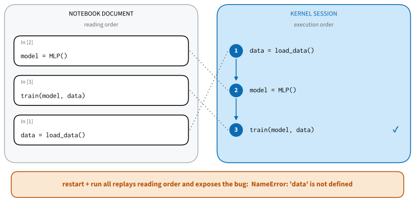
Figure 30.1.1 shows the classic failure. During an editing session you executed a data-loading cell first, then wrote a model-definition cell above it, and everything worked because the kernel already held data. The document now tells a story that never happened. A reader who runs the cells in the order shown — or you, tomorrow, after a restart — hits a NameError.
The execution counters (In [3], In [1], …) are historical clues, not a dependency graph. The following pair of cells demonstrates benign, document-ordered state: the second cell works only because the first ran.
-0.2638849576850524That dependency is fine, because it follows the reading order. A cell that depends on an assignment below it, or on a cell you have since deleted, is not. Keep cells small, keep function definitions separate from experiments, and pass data explicitly rather than mutating globals across many cells.
30.1.1.2 Restart and Run All
Restart kernel and run all cells discards the kernel’s accumulated state and replays the document from a blank slate, in reading order. It catches hidden state, missing setup, and order dependencies before a notebook is shared. Run it before saving, sharing, or committing a notebook. Every notebook in this book is built and tested with this procedure — the outputs you see on the website are produced by a clean top-to-bottom run.
30.1.2 Running the Book Locally
30.1.2.1 Setting Up
Download the notebook archive described in Installation, or clone the current sources from GitHub. The archive includes CPU and GPU uv environment files. From the extracted directory, create the environment once and launch JupyterLab through it:
uv sync --locked
uv run jupyter lab
Use the GPU lock file on a compatible NVIDIA system when the examples require it. The kernel selected inside a notebook must belong to the environment where the packages were installed. A Jupyter server can see many kernels; its own Python process does not determine which one executes your notebook.
30.1.2.2 A Quick Sanity Check
Before changing code, record a compact identity check:
import os
import platform
import sys

{
    "python": sys.executable.replace(os.path.expanduser("~"), "~"),
    "version": platform.python_version(),
    "working_directory": os.path.basename(os.getcwd()),
}
{'python': '~/d2l-neu/.venv-pytorch/bin/python',
'version': '3.12.3',
'working_directory': 'chapter_appendix-tools-for-deep-learning'}This catches the two most common setup mistakes in one cell: a kernel from the wrong environment (sys.executable points somewhere unexpected) and a notebook opened from a directory where relative data paths no longer resolve.
30.1.3 Working in an Editor
30.1.3.1 JupyterLab
JupyterLab combines a file browser, notebook editor, terminals, a text editor, debugger support, and a view of running kernels. The essentials are stable even as the interface evolves:
- Run a cell with
Shift+Enter; use a terminal tab foruv, Git, and inspecting files. - Select the kernel by environment name, then verify
sys.executable. - Interrupt a long computation before restarting. Restarting releases Python state and, normally, the accelerator memory owned by that process.
- Use Restart Kernel and Run All Cells before saving a result for others.
- Inspect the Running panel and stop kernels you no longer use — closing a browser tab does not necessarily stop its kernel, and an orphaned kernel can hold gigabytes of GPU memory.
30.1.3.2 VS Code
Visual Studio Code edits and runs .ipynb files with kernel selection, a variable inspector, cell-level debugging, and notebook-aware diffs. Open the repository as a folder, choose the interpreter created by uv, and select that interpreter as the notebook kernel.
When a notebook grows into a project, VS Code can navigate definitions, run tests, format code, and review Git diffs. Keep testable logic in .py modules and use the notebook for explanation and experiment records. This repository also includes a VS Code extension for the book’s authoring workflow — switching framework views, previewing slides, syncing edits back to the source — described in Section 30.8.
30.1.3.3 Debugging and Timing
Use the notebook debugger when the kernel supports it, or move a small failing call into a module and debug it in a terminal. Resist broad try/except blocks that print “failed”: they discard the exception type and location that diagnosis needs. For quick measurements, IPython’s magics are built in:
values = np.arange(100_000, dtype=np.float64)
%timeit values @ values
10.1 μs ± 302 ns per loop (mean ± std. dev. of 7 runs, 100,000 loops each)One caveat when timing accelerators: GPU operations are asynchronous, so a host-side timer may measure only the dispatch of work, not its completion. Synchronize explicitly (or use the framework’s benchmarking utilities), warm up compiled kernels first, and record the shapes, precision, device, and library versions alongside the number.
30.1.4 Remote Machines
Your editor, the notebook server, the kernel, and the accelerator need not be on the same machine. A common setup runs JupyterLab next to the GPU while you edit from a laptop.
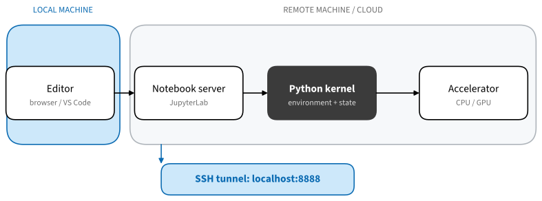
Bind the remote server to loopback and forward it over SSH:
# Remote machine
uv run jupyter lab --no-browser --ip 127.0.0.1 --port 8888
# Local machine
ssh -N -L 8888:127.0.0.1:8888 myserverThen open the tokenized http://127.0.0.1:8888/... URL locally. Never bind an unauthenticated Jupyter server to all network interfaces: anyone who can reach the port can execute code as you. The SSH tunnel provides encryption and access control; Jupyter’s token remains a useful second boundary.
VS Code’s Remote SSH installs a small server-side component so the editor UI runs locally while terminals, extensions, files, and kernels all live on the remote machine. Confirm the status bar shows SSH before selecting the Python environment — a local kernel cannot use the remote GPU. In either setup, treat remote compute as disposable: commit code and copy checkpoints to durable storage before it is rebooted, preempted, or deleted (Section 30.3).
Before sharing or committing a notebook, perform a final reproducibility and privacy check: restart and run all; check that setup does not rely on personal paths or unrecorded downloads; remove secrets and private data from outputs; keep the outputs that teach or verify something and delete noisy progress logs; and note the environment and hardware needed to interpret any measurement.
30.1.5 Summary
- Notebooks interleave prose, code, and results, and retain expensive state between experiments. Run and edit them rather than treating them as static documents.
- The document and the kernel hold different state in different orders; restart and run all is the test that they agree.
- Launch JupyterLab from the book’s
uvenvironment, and verify the kernel withsys.executablebefore trusting any result. - JupyterLab integrates notebooks, terminals, and kernels; VS Code adds modules, tests, diffs, and first-class remote development.
- Use SSH tunneling or VS Code Remote SSH instead of exposing a notebook server to the network.
30.1.6 Exercises
- Create an intentional out-of-order dependency like the one in Figure 30.1.1, confirm that it works interactively, and then detect it with restart and run all.
- Compare
sys.executablein a terminal, a JupyterLab kernel, and a VS Code kernel on your machine. Explain any difference. - Time a matrix product with
%timeiton CPU and, if available, on a GPU with and without synchronization. Explain the discrepancy. - Connect to a remote machine through an SSH tunnel and identify where the editor, server, kernel, and file system each run.