%matplotlib inline
from d2l import torch as d2l
import gymnasium as gym
import numpy as np14.2 Dynamic Programming
When the state space, action space, transition kernel, and reward are known, an optimal policy can be computed by dynamic programming (Bellman 1957). The Bellman equations decompose each state’s value into its immediate reward and the values of possible successor states. For discounted finite MDPs, the associated Bellman operator is a contraction, which yields a unique solution and a convergent iterative algorithm. We apply these results to FrozenLake and compare the optimal policy with the shortest-path policy.
%matplotlib inline
from d2l import jax as d2l
import gymnasium as gym
import numpy as np
14.2.1 Policies and Value Functions
14.2.1.1 State Values and Action Values
A stochastic policy \(\pi(a \mid s)\) (policy for short) is a conditional distribution over the actions \(a \in \mathcal{A}\) given the state \(s \in \mathcal{S}\): at some state of the lake the probabilities of left, down, right, up might be \((0.4, 0.2, 0.1, 0.3)\). A deterministic policy puts all its probability on a single action, which we then call \(\pi(s)\); more generally we abbreviate the distribution \(\pi(\cdot \mid s)\) as \(\pi(s)\).
For a fixed policy, an agent starting from \(s_0\) samples \(a_t \sim \pi(s_t)\), moves to \(s_{t+1} \sim P(\cdot \mid s_t, a_t)\), and traces out the trajectory \(\tau\) of Section 14.1. Different runs give different trajectories, so the natural score is the average,
\[V^\pi(s_0) = E_{a_t \sim \pi(s_t),\ s_{t+1} \sim P(\cdot \mid s_t, a_t)} \Big[ \sum_{t=0}^\infty \gamma^t r(s_t, a_t) \Big], \tag{14.2.1}\]
the value function of \(\pi\). Because the start state is arbitrary, \(V^\pi\) assigns a number to every state. The algorithms below operate on this value table.
In implementations, it is often useful to maintain a closely related quantity called the “action value” function. This is defined as the average return of a trajectory that begins at \(s_0\) but whose first-stage action is fixed to be \(a_0\)
\[Q^\pi(s_0, a_0) = r(s_0, a_0) + E_{a_t \sim \pi(s_t),\ s_{t+1} \sim P(\cdot \mid s_t, a_t)} \Big[ \sum_{t=1}^\infty \gamma^t r(s_t, a_t) \Big], \tag{14.2.2}\]
note that the summation inside the expectation is from \(t=1,\ldots, \infty\) because the reward of the first stage is fixed in this case: act as you must for one step, then follow the policy forever.
14.2.1.2 The Identity Linking \(V\) and \(Q\)
The value function averages the action-value function over the policy’s first action:
\[V^\pi(s) = \sum_{a \in \mathcal{A}} \pi(a \mid s)\, Q^\pi(s, a);\ \textrm{for all } s \in \mathcal{S}. \tag{14.2.3}\]
Conversely, the first stage of \(Q^\pi\) is explicit: \(Q^\pi(s, a) = r(s, a) + \gamma \sum_{s'} P(s' \mid s, a) V^\pi(s')\). Because \(V^\pi(s)\) is a convex combination of \(Q^\pi(s, a)\) over actions, \(\max_a Q^\pi(s, a) \geq V^\pi(s)\). The inequality is strict when the policy assigns positive probability to actions below the maximum. Policy-improvement methods increase probability on actions with positive advantage.
14.2.1.3 The Advantage Function
The advantage of an action is its value relative to the policy’s average value at that state,
\[ A^\pi(s, a) = Q^\pi(s, a) - V^\pi(s), \qquad E_{a \sim \pi(s)} \big[ A^\pi(s, a) \big] = 0, \tag{14.2.4}\]
The zero-mean identity follows directly from the relation between \(V^\pi\) and \(Q^\pi\). A positive advantage indicates that action \(a\) performs better than the policy’s current average at state \(s\). Later policy-gradient methods estimate or approximate this quantity when updating the policy.
14.2.2 The Bellman Equations
The Markov assumption converts the infinite trajectory sums above into local recursive equations.
14.2.2.1 The Expectation Form
Separate a trajectory after its first transition. The first part contains action \(a_0\), reward \(r(s_0,a_0)\), and next state \(s_1\); the remainder is the trajectory beginning at \(s_1\). By the Markov property, the expected return of the remainder depends on the past only through \(s_1\) and equals \(V^\pi(s_1)\). The value at \(s_0\) is therefore the expected immediate reward plus the discounted expected value of the next state:
\[V^\pi(s_0) = E_{a_0 \sim \pi(s_0)} \Big[ r(s_0, a_0) + \gamma\ E_{s_1 \sim P(s_1 \mid s_0, a_0)} \Big[ V^\pi(s_1) \Big] \Big]. \tag{14.2.5}\]
This decomposition is the basis of dynamic programming and of the Bellman updates used by many reinforcement-learning algorithms. The outer expectation averages over the policy’s choice of \(a_0\); the inner one averages over the environment’s next state \(s_1\) conditional on that action. For finite state and action spaces, we can write these expectations as sums:
\[V^\pi(s) = \sum_{a \in \mathcal{A}} \pi(a \mid s) \Big[ r(s, a) + \gamma\ \sum_{s' \in \mathcal{S}} P(s' \mid s, a) V^\pi(s') \Big];\ \textrm{for all } s \in \mathcal{S}. \tag{14.2.6}\]
The same decomposition applies to a trajectory beginning at any state \(s\in\mathcal{S}\). Conditioning additionally on the first action gives the corresponding equation for the action value:
\[Q^\pi(s, a) = r(s, a) + \gamma \sum_{s' \in \mathcal{S}} P(s' \mid s, a) \sum_{a' \in \mathcal{A}} \pi(a' \mid s')\ Q^\pi(s', a');\ \textrm{ for all } s \in \mathcal{S}, a \in \mathcal{A}. \tag{14.2.7}\]
This version is the analog of Equation 14.2.6 for the action value function. These are the Bellman expectation equations: for a fixed policy, Equation 14.2.6 is a system of \(|\mathcal{S}|\) linear equations in \(|\mathcal{S}|\) unknowns. The infinite horizon has disappeared into the recursion.
14.2.2.2 The Optimality Equation
An optimal policy maximizes the value function. We may write \(\pi^* = \mathrm{argmax}_\pi V^\pi(s_0)\) for a chosen start state. For a discounted finite MDP, however, one stationary deterministic policy is optimal from every state.
Proposition (a uniformly optimal policy exists). In a finite MDP with discount \(0 \leq \gamma < 1\) there is a deterministic, stationary policy \(\pi^*\) that is optimal at every state simultaneously: \(V^{\pi^*}(s) \geq V^\pi(s)\) for all \(s \in \mathcal{S}\) and all policies \(\pi\), including stochastic and history-dependent ones (Puterman 1994).
The intuition is the two-stage decomposition itself: what is best at a state does not depend on how the agent arrived there, so the best behaviors from different starts never conflict; and randomizing cannot help, since a convex combination of action values never exceeds their maximum. Write \(V^* \equiv V^{\pi^*}\) and \(Q^* \equiv Q^{\pi^*}\), and insert \(\pi^*\) into Equation 14.2.6: the policy assigns probability only to maximizing actions, so the average becomes a maximum,
\[V^*(s) = \max_{a \in \mathcal{A}} \Big[ r(s, a) + \gamma\ \sum_{s' \in \mathcal{S}} P(s' \mid s, a)\ V^*(s') \Big];\ \textrm{for all } s \in \mathcal{S}. \tag{14.2.8}\]
This is the Bellman optimality equation (Bellman 1952, 1957). Its optimal-substructure property says that after any first transition, the continuation must itself be optimal from the resulting state. Unlike the expectation form, it mentions no policy: it is an equation in the unknown table \(V^*\) and is nonlinear because of the maximum. Given its solution, a maximizing action follows from one model-based lookahead:
\[\pi^*(s) = \underset{a \in \mathcal{A}}{\mathrm{argmax}} \Big[ r(s, a) + \gamma \sum_{s' \in \mathcal{S}} P(s' \mid s, a)\ V^*(s') \Big]. \tag{14.2.9}\]
For a deterministic policy, the optimal action at state \(s\) maximizes its immediate reward \(r(s, a)\) plus the discounted expected value over possible next states \(s'\). The next state \(s'\) is averaged according to the transition model. The action-value version of Equation 14.2.8 is
\[Q^*(s, a) = r(s, a) + \gamma \sum_{s' \in \mathcal{S}} P(s' \mid s, a) \max_{a' \in \mathcal{A}} Q^*(s', a'),\]
The distinction matters for Section 14.4: extracting \(\pi^*(s) = \mathrm{argmax}_a Q^*(s, a)\) from \(Q^*\) needs no additional model, whereas extraction from \(V^*\) via Equation 14.2.9 uses \(P\) and \(r\) in the lookahead.
14.2.2.3 Backup Diagrams
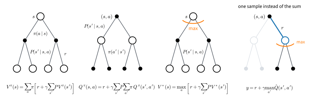
The four equations share a common structure: the value at a root is computed from values one step below it. Such updates are called backups; Figure 14.2.1 illustrates them. The sampled update in Section 14.4 replaces the expectation over next states with the single observed transition shown in blue in the rightmost diagram.
14.2.3 Convergence via Contraction
The Bellman optimality equation defines \(V^*\) implicitly. To compute it, read Equation 14.2.8 as a map: the Bellman optimality operator \(T\) acts on any table \(V: \mathcal{S} \to \mathbb{R}\) by
\[(TV)(s) = \max_{a \in \mathcal{A}} \Big[ r(s, a) + \gamma \sum_{s' \in \mathcal{S}} P(s' \mid s, a)\ V(s') \Big], \tag{14.2.10}\]
so that Equation 14.2.8 says exactly \(V^* = TV^*\): the optimal value function is a fixed point of \(T\). The operator \(T\) contracts distances in the sup norm.
14.2.3.1 The Contraction Proposition
Distance between value functions is measured in the sup norm \(\|V\|_\infty = \max_{s} |V(s)|\), the largest disagreement at any state.
Proposition (the Bellman operator is a \(\gamma\)-contraction). For any two tables \(V, V': \mathcal{S} \to \mathbb{R}\),
\[\|TV - TV'\|_\infty \leq \gamma\, \|V - V'\|_\infty. \tag{14.2.11}\]
Proof. Fix \(s\) and write \(f(a)\) and \(g(a)\) for the bracketed terms in \((TV)(s)\) and \((TV')(s)\). For every \(a\), \(|f(a) - g(a)| = \gamma\, |\sum_{s'} P(s' \mid s, a)(V(s') - V'(s'))| \leq \gamma \|V - V'\|_\infty\), because the probabilities are non-negative and sum to one. The difference between two maxima is bounded by the largest input difference, \(|\max_a f(a) - \max_a g(a)| \leq \max_a |f(a) - g(a)|\), so \(|(TV)(s) - (TV')(s)| \leq \gamma \|V - V'\|_\infty\) for every \(s\). \(\blacksquare\)
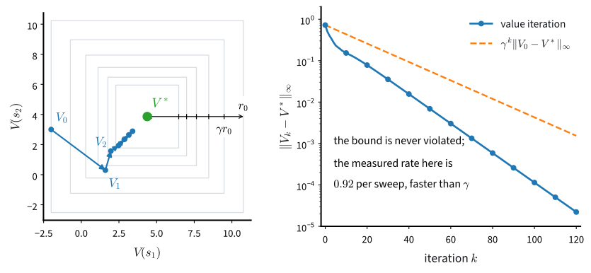
The contraction permits an application of Banach’s fixed-point theorem. It implies that the Bellman operator has a unique fixed point and that repeated application converges to it. Figure 14.2.2 illustrates the resulting nested error bounds.
14.2.3.2 Consequences of Contraction
The contraction has four consequences. First, the fixed point is unique: if \(V\) and \(V'\) are fixed points, then \(\|V-V'\|_\infty\leq\gamma\|V-V'\|_\infty\), which for \(\gamma<1\) implies \(V=V'\). Second, value iteration converges from any initial \(V_0\) at a geometric rate:
\[\|V_k - V^*\|_\infty = \|TV_{k-1} - TV^*\|_\infty \leq \gamma\, \|V_{k-1} - V^*\|_\infty \leq \cdots \leq \gamma^k\, \|V_0 - V^*\|_\infty, \tag{14.2.12}\]
Thus accuracy \(\varepsilon\) is reached after at most \(\log(\|V_0-V^*\|_\infty/\varepsilon)/\log(1/\gamma)\) sweeps. For \(\gamma\) near one, the denominator is approximately \(1-\gamma\), connecting the rate to the effective horizon of Section 14.1. Third, the successive differences provide a computable stopping rule:
\[\|V_k - V^*\|_\infty \leq \frac{\gamma}{1 - \gamma}\, \|V_k - V_{k-1}\|_\infty, \tag{14.2.13}\]
The right-hand side depends only on consecutive iterates. Fourth, when \(\gamma=1\) the operator is no longer a strict contraction, so uniqueness and convergence do not follow from this argument. Some episodic undiscounted problems still converge, but the general guarantee is absent. Replacing the maximum by an expectation under a fixed policy gives the policy-evaluation operator \(T^\pi\), which is a contraction by the same proof and has fixed point \(V^\pi\) (Puterman 1994; Bertsekas 2025).
14.2.4 Value Iteration, Policy Evaluation and Policy Iteration
Repeated application of the Bellman operator gives value iteration. We apply it to the slippery FrozenLake model from Section 14.1:
gamma = 0.95
LEFT, DOWN, RIGHT, UP = 0, 1, 2, 3
env = gym.make('FrozenLake-v1', is_slippery=True)
mdp = d2l.TabularMDP.from_gym(env, gamma)
gamma = 0.95
LEFT, DOWN, RIGHT, UP = 0, 1, 2, 3
env = gym.make('FrozenLake-v1', is_slippery=True)
mdp = d2l.TabularMDP.from_gym(env, gamma)14.2.4.1 Value Iteration
Iterate the operator: initialize \(V_0\) arbitrarily (we use zeros) and sweep
\[V_{k+1}(s) = \max_{a \in \mathcal{A}} \Big[ r(s, a) + \gamma\ \sum_{s' \in \mathcal{S}} P(s' \mid s, a)\ V_k(s') \Big];\ \textrm{for all } s \in \mathcal{S}, \tag{14.2.14}\]
that is, \(V_{k+1} = TV_k\). This is value iteration. The contraction result implies that \(V_k \to V^*\) from any initialization at geometric rate \(\gamma\). In code the sweep is one line, because mdp.backup from Section 14.1 computes the bracket for every state-action pair at once:
def value_iteration(mdp, num_iters):
    """Sweep V <- max_a backup(V); return the whole history of iterates."""
    V, history = np.zeros(mdp.num_states), []
    for _ in range(num_iters):
        V = mdp.backup(V).max(axis=1)
        history.append(V)
    return np.array(history)
def value_iteration(mdp, num_iters):
"""Sweep V <- max_a backup(V); return the whole history of iterates."""
V, history = np.zeros(mdp.num_states), []
for _ in range(num_iters):
V = mdp.backup(V).max(axis=1)
history.append(V)
return np.array(history)Value iteration is the chapter’s explicit model-based planning algorithm: it uses the transition and reward arrays directly. The model-free methods introduced next use sampled transitions instead. We run value iteration past the stopping tolerance, keep the final iterate as \(V^*\), and extract the policy by the greedy lookahead Equation 14.2.9:
history = value_iteration(mdp, num_iters=1000)
V_star = history[-1]
pi_star = mdp.backup(V_star).argmax(axis=1)
print(f'V*(s0) = {V_star[0]:.4f}')
d2l.show_grid(env.unwrapped.desc, V_star, pi_star)
V*(s0) = 0.1805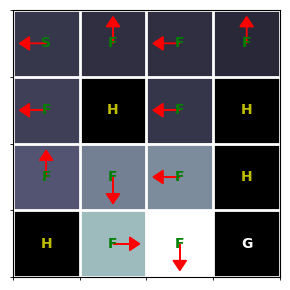
history = value_iteration(mdp, num_iters=1000)
V_star = history[-1]
pi_star = mdp.backup(V_star).argmax(axis=1)
print(f'V*(s0) = {V_star[0]:.4f}')
d2l.show_grid(env.unwrapped.desc, V_star, pi_star)
V*(s0) = 0.1805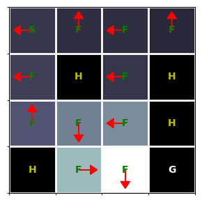
The values increase from about \(0.18\) at the start to \(0.72\) beside the goal. On deterministic ice, the shortest route would give the start state value \(\gamma^5\approx0.774\); stochastic slips reduce that value by roughly three quarters even under the optimal policy. Several optimal actions point away from the goal. We interpret them below after checking the predicted convergence rate:
err = np.concatenate([[np.abs(V_star).max()],
                      np.abs(history - V_star).max(axis=1)])
k = np.arange(131)
assert (err[k] <= err[0] * gamma ** k + 1e-12).all()
d2l.plot_curves({'value iteration': np.log10(err[k]),
                 'gamma^k guarantee': np.log10(err[0] * gamma ** k)},
                xlabel='sweep k', ylabel='log10 of sup-norm distance to V*')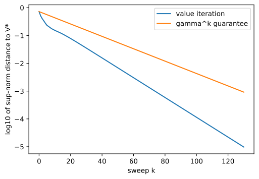
err = np.concatenate([[np.abs(V_star).max()],
                      np.abs(history - V_star).max(axis=1)])
k = np.arange(131)
assert (err[k] <= err[0] * gamma ** k + 1e-12).all()
d2l.plot_curves({'value iteration': np.log10(err[k]),
                 'gamma^k guarantee': np.log10(err[0] * gamma ** k)},
                xlabel='sweep k', ylabel='log10 of sup-norm distance to V*')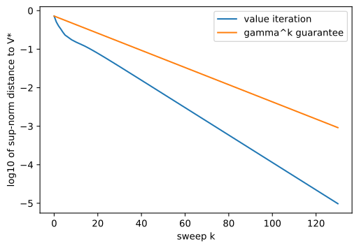
On the logarithmic scale, geometric decay appears as a straight line. The guarantee contracts by \(\gamma=0.95\) per sweep, whereas the measured error contracts by about \(0.92\). The bound reaches \(10^{-6}\) at sweep 263, and the measured error reaches it at sweep 158. Thus the discount factor, through the effective horizon, governs the worst-case sweep count; neither the number of cells nor their distance from the goal appears in the contraction rate. An implementation cannot observe the true error and must instead use a stopping criterion:
gap = np.abs(np.diff(history, axis=0)).max(axis=1)
true_err = np.abs(history[1:] - V_star).max(axis=1)
certified = gamma / (1 - gamma) * gap
assert (true_err <= certified + 1e-12).all()
for name, e in [('sweep-to-sweep change', gap),
                ('certified error bound', certified),
                ('distance to V*', true_err)]:
    print(f'{name} first below 1e-6 at sweep {np.argmax(e <= 1e-6) + 2}')
k_cert = np.argmax(certified <= 1e-6) + 2
sweep-to-sweep change first below 1e-6 at sweep 128
certified error bound first below 1e-6 at sweep 164
distance to V* first below 1e-6 at sweep 158gap = np.abs(np.diff(history, axis=0)).max(axis=1)
true_err = np.abs(history[1:] - V_star).max(axis=1)
certified = gamma / (1 - gamma) * gap
assert (true_err <= certified + 1e-12).all()
for name, e in [('sweep-to-sweep change', gap),
('certified error bound', certified),
('distance to V*', true_err)]:
print(f'{name} first below 1e-6 at sweep {np.argmax(e <= 1e-6) + 2}')
k_cert = np.argmax(certified <= 1e-6) + 2sweep-to-sweep change first below 1e-6 at sweep 128
certified error bound first below 1e-6 at sweep 164
distance to V* first below 1e-6 at sweep 158The unadjusted rule \(\|V_{k+1}-V_k\|_\infty<10^{-6}\) stops at sweep \(128\) but does not directly bound the error to \(V^*\). The contraction-based certificate stops at sweep \(164\), while the actual error first falls below \(10^{-6}\) at sweep \(158\). Thus the certified rule is conservative by six sweeps in this example.
14.2.4.2 Policy Evaluation
Replace the max in Equation 14.2.14 by the policy’s own average and the same iteration computes the value of any fixed policy \(\pi\):
\[V^\pi_{k+1}(s) = \sum_{a \in \mathcal{A}} \pi(a \mid s) \Big[ r(s, a) + \gamma\ \sum_{s' \in \mathcal{S}} P(s' \mid s, a)\ V^\pi_k(s') \Big];\ \textrm{for all } s \in \mathcal{S}. \tag{14.2.15}\]
This is policy evaluation, the fixed-point iteration for \(T^\pi\), convergent from any initialization because \(T^\pi\) contracts too. With the max gone the equations are linear, so they can also be solved directly, as Section 14.1 did with np.linalg.solve; the sweep does the same work one contraction at a time, and is the form that generalizes beyond tables.
def policy_evaluation(mdp, pi, num_iters):
    """Same sweep with the max replaced by an average under pi(a|s)."""
    V, history = np.zeros(mdp.num_states), []
    for _ in range(num_iters):
        V = (pi * mdp.backup(V)).sum(axis=1)
        history.append(V)
    return np.array(history)

uniform = np.ones((mdp.num_states, mdp.num_actions)) / mdp.num_actions
print(f'V(s0) for the uniformly random policy: '
      f'{policy_evaluation(mdp, uniform, 400)[-1][0]:.4f}')
V(s0) for the uniformly random policy: 0.0078def policy_evaluation(mdp, pi, num_iters):
"""Same sweep with the max replaced by an average under pi(a|s)."""
V, history = np.zeros(mdp.num_states), []
for _ in range(num_iters):
V = (pi * mdp.backup(V)).sum(axis=1)
history.append(V)
return np.array(history)
uniform = np.ones((mdp.num_states, mdp.num_actions)) / mdp.num_actions
print(f'V(s0) for the uniformly random policy: '
f'{policy_evaluation(mdp, uniform, 400)[-1][0]:.4f}')V(s0) for the uniformly random policy: 0.0078The uniformly random policy of Section 14.1 reaches the goal in very few episodes. Its start-state value is \(0.0078\), about four percent of the optimum. Policy evaluation measures performance without improving the policy; learned critics in Section 15.1 approximate the same value computation from sampled data.
14.2.4.3 Policy Iteration and Generalized Policy Iteration
Evaluation plus the greedy step Equation 14.2.9 suggests a different algorithm: evaluate the current policy fully, act greedily on its value function, repeat. The following policy-improvement proposition justifies the greedy step.
Proposition (policy improvement). Let \(\pi\) be any policy and let \(\pi'\) be greedy with respect to \(V^\pi\), that is \(\pi'(s) = \mathrm{argmax}_a \big[ r(s, a) + \gamma \sum_{s'} P(s' \mid s, a) V^\pi(s') \big]\). Then \(V^{\pi'}(s) \geq V^\pi(s)\) at every state, and if equality holds everywhere then both policies are optimal.
Proof. Greediness says one step of \(\pi'\) is at least as good as one step of \(\pi\): \(T^{\pi'} V^\pi = T V^\pi \geq T^\pi V^\pi = V^\pi\). The operator \(T^{\pi'}\) is monotone (its coefficients are probabilities), so \(V^\pi \leq T^{\pi'} V^\pi \leq (T^{\pi'})^2 V^\pi \leq \cdots \to V^{\pi'}\), the limit being \(T^{\pi'}\)’s unique fixed point. If \(V^{\pi'} = V^\pi\), the first line reads \(TV^\pi = V^\pi\), so \(V^\pi\) solves the optimality equation and uniqueness finishes the job. \(\blacksquare\)
Each round of policy iteration therefore strictly improves the policy until it is optimal, and a finite MDP has finitely many deterministic policies, so termination is guaranteed (Puterman 1994). The implementation alternates evaluation and improvement until the policy stops changing:
pi, num_outer = uniform, 0
while True:
    V = policy_evaluation(mdp, pi, 800)[-1]                # evaluate pi
    new = np.eye(mdp.num_actions)[mdp.backup(V).argmax(axis=1)]  # improve
    num_outer += 1
    if (new == pi).all():                                  # nothing changed
        break
    pi = new
assert np.abs(V - V_star).max() < 1e-12
pi, num_outer = uniform, 0
while True:
V = policy_evaluation(mdp, pi, 800)[-1] # evaluate pi
new = np.eye(mdp.num_actions)[mdp.backup(V).argmax(axis=1)] # improve
num_outer += 1
if (new == pi).all(): # nothing changed
break
pi = new
assert np.abs(V - V_star).max() < 1e-12The assertion verifies that value iteration and policy iteration agree on \(V^*\) to twelve decimal places. Their computational costs, however, are organized differently:
ok = [(mdp.backup(V).argmax(axis=1) == pi_star).all() for V in history]
print(f'policy iteration: {num_outer} rounds of evaluate-then-improve')
print(f'value iteration: certified at sweep {k_cert}')
print(f'its greedy policy already equals pi* from sweep '
      f'{np.argmax(ok) + 1} on')
policy iteration: 2 rounds of evaluate-then-improve
value iteration: certified at sweep 164
its greedy policy already equals pi* from sweep 14 onok = [(mdp.backup(V).argmax(axis=1) == pi_star).all() for V in history]
print(f'policy iteration: {num_outer} rounds of evaluate-then-improve')
print(f'value iteration: certified at sweep {k_cert}')
print(f'its greedy policy already equals pi* from sweep '
f'{np.argmax(ok) + 1} on')policy iteration: 2 rounds of evaluate-then-improve
value iteration: certified at sweep 164
its greedy policy already equals pi* from sweep 14 onPolicy iteration requires two improvement rounds on this example, but each round contains 800 evaluation sweeps. Bellman backups therefore provide a more informative comparison than outer iterations. For value iteration, the greedy policy becomes optimal at sweep 14, well before the value-error certificate is satisfied. The policy depends only on the ordering of action values, so it can stabilize before their numerical values have converged.
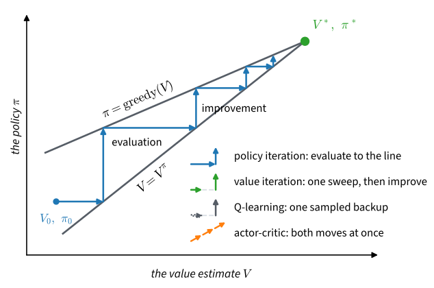
Policy evaluation and improvement need not be completed in separate phases. Generalized policy iteration (GPI) interleaves updates that move \(V\) toward \(V^\pi\) with updates that move \(\pi\) toward a greedy policy (Sutton and Barto 2018). Policy iteration performs nearly complete evaluation before improvement, whereas value iteration improves after each sweep. Q-learning uses sampled backups (Section 14.4), and actor–critic methods update value and policy estimates together (Section 15.1). Figure 14.2.3 summarizes these cases.
14.2.4.4 The Optimal Policy on Slippery Ice
Although \(\pi^*\) maximizes expected return, some of its actions point away from the goal. We evaluate policies by their mean return over sampled episodes without using the transition model:
def evaluate(env, policy, num_episodes, gamma=1.0, rng=None):
    """Mean discounted return of an acting policy over Monte Carlo episodes.

    `policy(obs, rng) -> action` is the protocol every agent in these two
    chapters speaks; a deterministic policy simply ignores `rng`."""
    total = 0.0
    for _ in range(num_episodes):
        obs, done, discount = env.reset()[0], False, 1.0
        while not done:
            obs, reward, terminated, truncated, _ = env.step(policy(obs, rng))
            done = terminated or truncated
            total, discount = total + discount * reward, discount * gamma
    return total / num_episodes
def evaluate(env, policy, num_episodes, gamma=1.0, rng=None):
"""Mean discounted return of an acting policy over Monte Carlo episodes.
`policy(obs, rng) -> action` is the protocol every agent in these two
chapters speaks; a deterministic policy simply ignores `rng`."""
total = 0.0
for _ in range(num_episodes):
obs, done, discount = env.reset()[0], False, 1.0
while not done:
obs, reward, terminated, truncated, _ = env.step(policy(obs, rng))
done = terminated or truncated
total, discount = total + discount * reward, discount * gamma
return total / num_episodesThe evaluation protocol represents a policy as a function from observation to action, optionally using an explicit random generator. Later sections use the same interface. With the default \(\gamma = 1\) and terminal-only reward, the mean return is the success rate. We compare \(\pi^*\) with the shortest-path policy derived for deterministic ice:
shortest = np.array([DOWN, RIGHT, DOWN, LEFT,
                     DOWN, LEFT, DOWN, LEFT,
                     RIGHT, DOWN, DOWN, LEFT,
                     LEFT, RIGHT, RIGHT, LEFT])   # optimal on calm ice, by hand
env.reset(seed=0)
for name, p in [('slip-aware optimum', pi_star),
                ('shortest-path policy', shortest)]:
    success = evaluate(env, lambda s, _: int(p[s]), num_episodes=2000)
    print(f'{name}: reaches the goal in {success:.1%} of 2000 episodes')
slip-aware optimum: reaches the goal in 73.6% of 2000 episodes
shortest-path policy: reaches the goal in 4.7% of 2000 episodesshortest = np.array([DOWN, RIGHT, DOWN, LEFT,
DOWN, LEFT, DOWN, LEFT,
RIGHT, DOWN, DOWN, LEFT,
LEFT, RIGHT, RIGHT, LEFT]) # optimal on calm ice, by hand
env.reset(seed=0)
for name, p in [('slip-aware optimum', pi_star),
('shortest-path policy', shortest)]:
success = evaluate(env, lambda s, _: int(p[s]), num_episodes=2000)
print(f'{name}: reaches the goal in {success:.1%} of 2000 episodes')slip-aware optimum: reaches the goal in 73.6% of 2000 episodes
shortest-path policy: reaches the goal in 4.7% of 2000 episodesThe dynamic-programming policy reaches the goal in about \(0.74\) of the episodes, compared with about \(0.05\) for the shortest-path policy. These rates count episodes that finish within the environment’s 100-step limit; without the limit, the success probability of the optimal policy is about \(0.78\). The shortest path places five of its six actions next to holes, where perpendicular slips can terminate the episode. The optimal policy takes a longer route that reduces this risk. The statewise differences are shown below:
row, col = np.arange(16) // 4, np.arange(16) % 4
to_row = np.clip(row + np.array([0, 1, 0, -1])[pi_star], 0, 3)
to_col = np.clip(col + np.array([-1, 0, 1, 0])[pi_star], 0, 3)
frozen = np.isin(env.unwrapped.desc.flatten(), [b'S', b'F'])
away = np.flatnonzero(frozen & ((3 - to_row) + (3 - to_col)
                                > (3 - row) + (3 - col)))
for s in away:
    print(f's={s:>2}: pi* commands {"<v>^"[pi_star[s]]}, '
          f'the shortest path takes {"<v>^"[shortest[s]]}')
s= 2: pi* commands <, the shortest path takes v
s= 6: pi* commands <, the shortest path takes v
s= 8: pi* commands ^, the shortest path takes >
s=10: pi* commands <, the shortest path takes vrow, col = np.arange(16) // 4, np.arange(16) % 4
to_row = np.clip(row + np.array([0, 1, 0, -1])[pi_star], 0, 3)
to_col = np.clip(col + np.array([-1, 0, 1, 0])[pi_star], 0, 3)
frozen = np.isin(env.unwrapped.desc.flatten(), [b'S', b'F'])
away = np.flatnonzero(frozen & ((3 - to_row) + (3 - to_col)
> (3 - row) + (3 - col)))
for s in away:
print(f's={s:>2}: pi* commands {"<v>^"[pi_star[s]]}, '
f'the shortest path takes {"<v>^"[shortest[s]]}')s= 2: pi* commands <, the shortest path takes v
s= 6: pi* commands <, the shortest path takes v
s= 8: pi* commands ^, the shortest path takes >
s=10: pi* commands <, the shortest path takes vAt four of the eleven nonterminal frozen cells, the optimal command points away from the goal. At state 8, up is the only action whose three possible outcomes all avoid the hole at state 12: the agent moves to state 4, state 9, or remains against the wall. At states 1 and 3, commanding up also uses the wall to avoid more dangerous outcomes. These choices follow from averaging over the three transition outcomes in Equation 14.2.9.
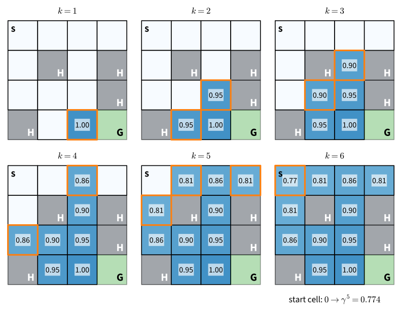
Deterministic case. Without slippery transitions, \(V^*(s)=\gamma V^*(s')\) along an optimal move. Hence \(V^*(s)=\gamma^{d(s)-1}\), where \(d(s)\) is the shortest distance to the goal. After \(k\) sweeps, value has propagated to exactly the states within \(k\) moves of the goal, and this map converges in six sweeps (Figure 14.2.4). This finite wavefront is specific to deterministic terminal rewards; the stochastic case converges geometrically. The greedy policy for the deterministic solution is exactly the shortest-path policy, as verified below.
calm = d2l.TabularMDP.from_gym(
    gym.make('FrozenLake-v1', is_slippery=False), gamma)
V_calm = value_iteration(calm, num_iters=10)[-1]
assert (calm.backup(V_calm).argmax(axis=1) == shortest).all()
print(f'V*(s0) on calm ice: {V_calm[0]:.4f};  gamma^5 = {gamma ** 5:.4f}')
V*(s0) on calm ice: 0.7738; gamma^5 = 0.7738calm = d2l.TabularMDP.from_gym(
gym.make('FrozenLake-v1', is_slippery=False), gamma)
V_calm = value_iteration(calm, num_iters=10)[-1]
assert (calm.backup(V_calm).argmax(axis=1) == shortest).all()
print(f'V*(s0) on calm ice: {V_calm[0]:.4f}; gamma^5 = {gamma ** 5:.4f}')V*(s0) on calm ice: 0.7738; gamma^5 = 0.7738The optimal start-state value decreases from \(0.774\) on deterministic ice to \(0.180\) on slippery ice. This difference quantifies the effect of the stochastic transitions under optimal play.
14.2.5 Summary
A policy is described by its state and action values, related by \(V^\pi(s)=\sum_a\pi(a\mid s)Q^\pi(s,a)\). The Bellman expectation equations characterize a fixed policy, and the Bellman optimality equation characterizes \(V^*\). For \(\gamma<1\), the optimality operator is a contraction: its fixed point is unique, value iteration converges geometrically, and consecutive iterates give a computable error bound. Policy evaluation replaces maximization by an expectation under a fixed policy. Policy iteration alternates evaluation with greedy improvement, while generalized policy iteration permits partial interleaving. These methods require the transition and reward model; later sections replace exact expectations by sampled transitions.
Experimental scope. The value functions, convergence counts, and policies are exact for this MDP at \(\gamma=0.95\). The two success rates are Monte Carlo estimates from \(2{,}000\) seeded episodes and vary slightly with the seed. The comparison demonstrates the value of planning with the correct stochastic model on this environment; it does not address learning when the model is unknown.
14.2.6 Exercises
- [short-code] Cost of a sweep. Give the cost of one value iteration sweep Equation 14.2.14 in terms of the number of states, the number of actions, and the number of successors per state-action pair, and say which of the three the dense
mdp.backupof Section 14.1 actually computes. Then use \(\|V_k - V^*\|_\infty \leq \gamma^k \|V_0 - V^*\|_\infty\) to show that reaching accuracy \(\varepsilon\) needs \(O(\log(1/\varepsilon) / \log(1/\gamma))\) sweeps. Confirm the per-sweep cost empirically (a few seconds) by timing the \(4 \times 4\) map against the \(8 \times 8\) map,d2l.TabularMDP.from_gym(gym.make('FrozenLake-v1', map_name='8x8', is_slippery=True), gamma). - [conceptual] The contraction, verified. The section’s proposition proved \(\|TV - TV'\|_\infty \leq \gamma \|V - V'\|_\infty\) using only that a maximum of differences bounds the difference of maxima. Re-derive the stopping rule \(\|V_k - V^*\|_\infty \leq \frac{\gamma}{1-\gamma} \|V_k - V_{k-1}\|_\infty\) from it by telescoping the tail \(\sum_{j \geq k} \|V_{j+1} - V_j\|_\infty\), and turn it into an \(\varepsilon\)-optimal stopping rule: how small must the sweep-to-sweep change be to guarantee an error below \(\varepsilon\)? Then walk through the proposition’s proof with \(\gamma = 1\) and point to the exact step that fails.
- [short-code] Predict, then run. Before running anything, predict \(V^*(s_0)\) on the calm map (
is_slippery=False) for \(\gamma \in \{0, 0.5, 0.9, 0.99\}\), and predict which of the four optimal policies differ. Now run value iteration for each and check. Explain in one sentence why the value depends on \(\gamma\) and the policy does not, and what is special about \(\gamma = 0\). - [short-code] Let the ice be calm. The section ran on slippery ice throughout. Switch the slip off, rerun value iteration, and compare the two optimal policies cell by cell. Which arrows change, and why does Equation 14.2.6 stop caring about the holes’ neighbors once \(P(s' \mid s, a)\) puts all its mass on the intended cell? The section printed \(V^*(s_0) = 0.180\) on ice and \(0.774\) calm, a ratio of about \(4.3\): is that larger or smaller than the naive reading “each commanded move now succeeds with probability \(1/3\)” suggests, and what does the difference show about how the optimal policy accounts for slips?
- [conceptual] When \(\gamma\) equals one. The contraction proposition needs \(\gamma < 1\), yet running the section’s code with \(\gamma = 1\) on FrozenLake converges. Explain why, using that the goal and the holes are absorbing and all rewards are non-negative, and say what the limit \(V_k(s)\) means in that case. Then construct a two-state MDP with a single action on which \(V_k\) grows without bound at \(\gamma = 1\), and verify it in three lines of code.
- [extended] Policy iteration measured in backups. Policy iteration converged in \(2\) rounds against value iteration’s \(164\) certified sweeps, which suggests a large advantage in outer iterations, but each round contained \(800\) evaluation sweeps of Equation 14.2.15 before the greedy step Equation 14.2.9. Measure both algorithms by the number of Bellman backups, and plot the sup-norm error against backups on the \(4 \times 4\) and \(8 \times 8\) maps (a few seconds each). Which converges in fewer outer iterations, which in fewer backups, and how does the answer move as \(\gamma \to 1\)? Does truncating the inner evaluation to ten sweeps change your accounting?