from d2l import torch as d2l
import torch
from torch import nn
from torch.nn import functional as F7.2 Blocks, Bottlenecks, and Branches: VGG, NiN, GoogLeNet
AlexNet demonstrated the effectiveness of deep convolutional networks, but its layers were designed individually. The next architectures introduced reusable organization. VGG (Simonyan and Zisserman 2015) made the repeated block the unit of design. Network in network (NiN) (Lin et al. 2013) mixed channels with \(1 \times 1\) convolutions and replaced fully connected classifiers by global average pooling. GoogLeNet (Szegedy et al. 2015) applied several convolution sizes in parallel within a multi-branch block and used the stem–body–head organization that remains common today.
import tensorflow as tf
from d2l import tensorflow as d2l
# Bound the JAX allocator while training several 224x224 models in one process;
# this setting does not change the model computation.
import os
os.environ['XLA_PYTHON_CLIENT_MEM_FRACTION'] = '.25'
from d2l import jax as d2l
from flax import nnx
from jax import numpy as jnp# Bound allocator and autotuning memory while training several 224x224 models
# in one process; these settings do not change the model computation.
import os
os.environ['MXNET_GPU_MEM_POOL_TYPE'] = 'Round'
os.environ['MXNET_CUDNN_AUTOTUNE_DEFAULT'] = '0'
from d2l import mxnet as d2l
from mxnet import np, npx, init
from mxnet.gluon import nn
npx.set_np()7.2.1 VGG: Blocks as the Unit of Design
VGG (Simonyan and Zisserman 2015) replaced individually chosen layers with repeated blocks. A block makes depth, channel count, and downsampling schedule explicit and lets code construct a network from a short configuration.
7.2.1.1 VGG Blocks
If every convolution is followed immediately by stride-2 pooling, an input of width \(d\) permits at most \(\lfloor\log_2 d\rfloor\) such stages before its spatial extent collapses. For a 224-pixel ImageNet input, this gives at most seven or eight stages, depending on boundary conventions. Depth can instead increase within a fixed resolution stage.
VGG places several stride-1 convolutions between pooling operations. Two stacked \(3 \times 3\) convolutions see the same \(5 \times 5\) window as one \(5 \times 5\) convolution while using \(18c^2\) rather than \(25c^2\) weights when input and output widths are both \(c\). Three layers cover a \(7 \times 7\) window with \(27c^2\) rather than \(49c^2\) weights, and insert a nonlinearity after every layer. The experiments of Simonyan and Zisserman (2015) found that these deeper configurations improved ImageNet accuracy under their training protocol. Small stacked kernels consequently became common and received specialized GPU implementations (Lavin and Gray 2016).
A VGG block therefore contains num_convs convolutions with \(3\times3\) kernels and padding 1, followed by \(2\times2\) max-pooling with stride 2. The function below takes the number of convolutions and their output channel count.
def vgg_block(num_convs, out_channels):
    layers = []
    for _ in range(num_convs):
        layers.append(nn.LazyConv2d(out_channels, kernel_size=3, padding=1))
        layers.append(nn.ReLU())
    layers.append(nn.MaxPool2d(kernel_size=2,stride=2))
    return nn.Sequential(*layers)
def vgg_block(num_convs, num_channels):
blk = tf.keras.models.Sequential()
for _ in range(num_convs):
blk.add(
tf.keras.layers.Conv2D(num_channels, kernel_size=3,
padding='same', activation='relu'))
blk.add(tf.keras.layers.MaxPool2D(pool_size=2, strides=2))
return blkdef vgg_block(num_convs, in_channels, out_channels, rngs):
layers = []
for _ in range(num_convs):
layers.append(nnx.Conv(in_channels, out_channels,
kernel_size=(3, 3), padding=(1, 1), rngs=rngs))
layers.append(nnx.relu)
in_channels = out_channels
layers.append(lambda x: nnx.max_pool(
x, window_shape=(2, 2), strides=(2, 2)))
return nnx.Sequential(*layers)def vgg_block(num_convs, num_channels):
blk = nn.Sequential()
for _ in range(num_convs):
blk.add(nn.Conv2D(num_channels, kernel_size=3,
padding=1, activation='relu'))
blk.add(nn.MaxPool2D(pool_size=2, strides=2))
return blk7.2.1.2 The VGG Network
Like AlexNet and LeNet, the VGG network can be partitioned into two parts: the first consisting mostly of convolutional and pooling layers and the second consisting of fully connected layers that are identical to those in AlexNet. The key difference is that the convolutional layers are grouped in nonlinear transformations that leave the dimensionality unchanged, followed by a resolution-reduction step, as depicted in Figure 7.2.1.
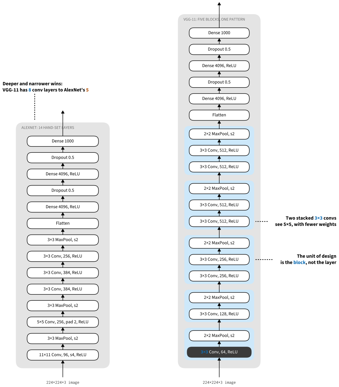
The convolutional part of the network connects several VGG blocks from Figure 7.2.1 (also defined in the vgg_block function) in succession. This grouping of convolutions is a pattern that has remained almost unchanged over the past decade, although the specific choice of operations has undergone considerable modifications. The variable arch consists of a list of tuples (one per block), where each contains two values: the number of convolutional layers and the number of output channels, which are precisely the arguments required to call the vgg_block function. As such, VGG defines a family of networks rather than just a specific manifestation. To build a specific network, we iterate over arch and compose the blocks.
class VGG(d2l.Classifier):
    def __init__(self, arch, lr=0.1, num_classes=10):
        super().__init__()
        self.save_hyperparameters()
        conv_blks = []
        for (num_convs, out_channels) in arch:
            conv_blks.append(vgg_block(num_convs, out_channels))
        self.net = nn.Sequential(
            *conv_blks, nn.Flatten(),
            nn.LazyLinear(4096), nn.ReLU(), nn.Dropout(0.5),
            nn.LazyLinear(4096), nn.ReLU(), nn.Dropout(0.5),
            nn.LazyLinear(num_classes))
        self.net.apply(d2l.init_cnn)
class VGG(d2l.Classifier):
def __init__(self, arch, lr=0.1, num_classes=10):
super().__init__()
self.save_hyperparameters()
self.net = tf.keras.models.Sequential()
for (num_convs, num_channels) in arch:
self.net.add(vgg_block(num_convs, num_channels))
self.net.add(
tf.keras.models.Sequential([
tf.keras.layers.Flatten(),
tf.keras.layers.Dense(4096, activation='relu'),
tf.keras.layers.Dropout(0.5),
tf.keras.layers.Dense(4096, activation='relu'),
tf.keras.layers.Dropout(0.5),
tf.keras.layers.Dense(num_classes)]))class VGG(d2l.Classifier):
def __init__(self, arch, lr=0.1, num_classes=10,
input_shape=(224, 224, 1), rngs=None):
super().__init__()
self.save_hyperparameters(ignore=['rngs'])
rngs = (nnx.Rngs(params=d2l.get_key(), dropout=d2l.get_key())
if rngs is None else rngs)
conv_blks = []
in_channels = input_shape[-1]
for num_convs, out_channels in arch:
conv_blks.append(vgg_block(
num_convs, in_channels, out_channels, rngs))
in_channels = out_channels
height, width = input_shape[:2]
flat_features = (height // 2 ** len(arch)) * (
width // 2 ** len(arch)) * in_channels
self.net = nnx.Sequential(
*conv_blks,
lambda x: x.reshape((x.shape[0], -1)), # flatten
nnx.Linear(flat_features, 4096, rngs=rngs), nnx.relu,
nnx.Dropout(0.5, rngs=rngs),
nnx.Linear(4096, 4096, rngs=rngs), nnx.relu,
nnx.Dropout(0.5, rngs=rngs),
nnx.Linear(4096, num_classes, rngs=rngs))class VGG(d2l.Classifier):
def __init__(self, arch, lr=0.1, num_classes=10):
super().__init__()
self.save_hyperparameters()
self.net = nn.Sequential()
for (num_convs, num_channels) in arch:
self.net.add(vgg_block(num_convs, num_channels))
self.net.add(nn.Dense(4096, activation='relu'), nn.Dropout(0.5),
nn.Dense(4096, activation='relu'), nn.Dropout(0.5),
nn.Dense(num_classes))
self.net.initialize(init.Xavier())The original VGG network had five convolutional blocks, among which the first two have one convolutional layer each and the latter three contain two convolutional layers each. The first block has 64 output channels and each subsequent block doubles the number of output channels, until that number reaches 512. Since this network uses eight convolutional layers and three fully connected layers, it is often called VGG-11.
VGG(arch=((1, 64), (1, 128), (2, 256), (2, 512), (2, 512))).layer_summary(
    (1, 1, 224, 224))
Sequential output shape: torch.Size([1, 64, 112, 112])
Sequential output shape: torch.Size([1, 128, 56, 56])
Sequential output shape: torch.Size([1, 256, 28, 28])
Sequential output shape: torch.Size([1, 512, 14, 14])
Sequential output shape: torch.Size([1, 512, 7, 7])
Flatten output shape: torch.Size([1, 25088])
Linear output shape: torch.Size([1, 4096])
ReLU output shape: torch.Size([1, 4096])
Dropout output shape: torch.Size([1, 4096])
Linear output shape: torch.Size([1, 4096])
ReLU output shape: torch.Size([1, 4096])
Dropout output shape: torch.Size([1, 4096])
Linear output shape: torch.Size([1, 10])VGG(arch=((1, 64), (1, 128), (2, 256), (2, 512), (2, 512))).layer_summary(
(1, 224, 224, 1))Sequential output shape: (1, 112, 112, 64)
Sequential output shape: (1, 56, 56, 128)
Sequential output shape: (1, 28, 28, 256)
Sequential output shape: (1, 14, 14, 512)
Sequential output shape: (1, 7, 7, 512)
Sequential output shape: (1, 10)VGG(arch=((1, 64), (1, 128), (2, 256), (2, 512), (2, 512)),
).layer_summary((1, 224, 224, 1))Sequential output shape: (1, 112, 112, 64)
Sequential output shape: (1, 56, 56, 128)
Sequential output shape: (1, 28, 28, 256)
Sequential output shape: (1, 14, 14, 512)
Sequential output shape: (1, 7, 7, 512)
function output shape: (1, 25088)
Linear output shape: (1, 4096)
custom_jvp output shape: (1, 4096)
Dropout output shape: (1, 4096)
Linear output shape: (1, 4096)
custom_jvp output shape: (1, 4096)
Dropout output shape: (1, 4096)
Linear output shape: (1, 10)VGG(arch=((1, 64), (1, 128), (2, 256), (2, 512), (2, 512))).layer_summary(
(1, 1, 224, 224))Sequential output shape: (1, 64, 112, 112)
Sequential output shape: (1, 128, 56, 56)
Sequential output shape: (1, 256, 28, 28)
Sequential output shape: (1, 512, 14, 14)
Sequential output shape: (1, 512, 7, 7)
Dense output shape: (1, 4096)
Dropout output shape: (1, 4096)
Dense output shape: (1, 4096)
Dropout output shape: (1, 4096)
Dense output shape: (1, 10)As you can see, we halve height and width at each block, finally reaching a height and width of 7 before flattening the representations for processing by the fully connected part of the network. Simonyan and Zisserman (2015) described several other variants of VGG. In fact, it has become the norm to propose families of networks with different speed–accuracy trade-offs when introducing a new architecture.
7.2.1.3 Training
Since VGG-11 is computationally more demanding than AlexNet we construct a network with a smaller number of channels. This is more than sufficient for training on Fashion-MNIST. The model training process is similar to that of AlexNet in Section 7.1. Again observe the close match between validation and training loss, suggesting only a small amount of overfitting.
model = VGG(arch=((1, 16), (1, 32), (2, 64), (2, 128), (2, 128)), lr=0.01)
trainer = d2l.Trainer(max_epochs=10, num_gpus=1)
data = d2l.FashionMNIST(batch_size=128, resize=(224, 224))
model.apply_init([next(iter(data.get_dataloader(True)))[0]], d2l.init_cnn)
trainer.fit(model, data)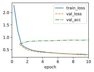
trainer = d2l.Trainer(max_epochs=10)
data = d2l.FashionMNIST(batch_size=128, resize=(224, 224))
with d2l.try_gpu():
    model = VGG(arch=((1, 16), (1, 32), (2, 64), (2, 128), (2, 128)), lr=0.01)
    trainer.fit(model, data)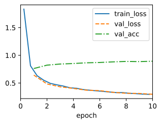
model = VGG(arch=((1, 16), (1, 32), (2, 64), (2, 128), (2, 128)), lr=0.01)
trainer = d2l.Trainer(max_epochs=10, num_gpus=1)
data = d2l.FashionMNIST(batch_size=128, resize=(224, 224))
trainer.fit(model, data)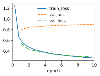
model = VGG(arch=((1, 16), (1, 32), (2, 64), (2, 128), (2, 128)), lr=0.01)
trainer = d2l.Trainer(max_epochs=10, num_gpus=1)
data = d2l.FashionMNIST(batch_size=128, resize=(224, 224))
trainer.fit(model, data)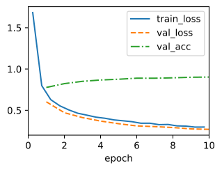
VGG established several durable design patterns: repeated convolutional blocks, deeper and narrower networks, and a family of models specified by block parameters. Varying those parameters exposes trade-offs between computational cost and accuracy.
7.2.2 NiN: \(1 \times 1\) Convolutions and Global Average Pooling
LeNet, AlexNet, and VGG all share a common design pattern: extract features exploiting spatial structure via a sequence of convolutions and pooling layers and post-process the representations via fully connected layers. The improvements upon LeNet by AlexNet and VGG mainly lie in how these later networks widen and deepen these two modules.
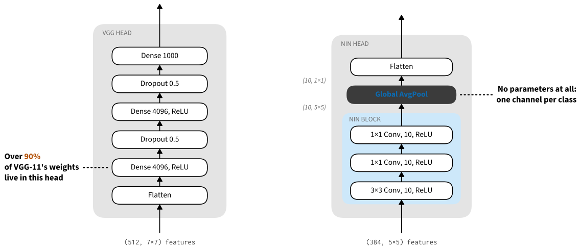
This design poses two challenges. First, the fully connected head contains many parameters: in VGG-11, the matrix for its first fully connected layer alone occupies almost 400 MB in single precision (FP32). This cost can rule out deployment on memory-constrained devices. Second, inserting fully connected layers earlier would discard spatial structure and require even more parameters.
The network in network (NiN) blocks (Lin et al. 2013) offer an alternative, capable of solving both problems in one simple strategy: (i) use \(1 \times 1\) convolutions to add local nonlinearities across the channel activations and (ii) use global average pooling to integrate across all locations in the last representation layer. Note that global average pooling would not be effective, were it not for the added nonlinearities.
7.2.2.1 NiN Blocks
Recall from Section 6.4.3 that a \(1 \times 1\) convolution is a fully connected layer applied independently at each pixel location: it mixes channels while leaving the spatial structure untouched. The idea behind NiN is to apply such a per-pixel fully connected layer after each ordinary convolution, twice, with ReLUs in between. This gives the network local nonlinear computation across channels at no spatial cost. Figure 7.2.2 illustrates the main structural differences between VGG and NiN, and their blocks.
def nin_block(out_channels, kernel_size, strides, padding):
    return nn.Sequential(
        nn.LazyConv2d(out_channels, kernel_size, strides, padding), nn.ReLU(),
        nn.LazyConv2d(out_channels, kernel_size=1), nn.ReLU(),
        nn.LazyConv2d(out_channels, kernel_size=1), nn.ReLU())
def nin_block(out_channels, kernel_size, strides, padding):
return tf.keras.models.Sequential([
tf.keras.layers.Conv2D(out_channels, kernel_size, strides=strides,
padding=padding),
tf.keras.layers.Activation('relu'),
tf.keras.layers.Conv2D(out_channels, 1),
tf.keras.layers.Activation('relu'),
tf.keras.layers.Conv2D(out_channels, 1),
tf.keras.layers.Activation('relu')])def nin_block(in_channels, out_channels, kernel_size, strides, padding, rngs):
return nnx.Sequential(
nnx.Conv(in_channels, out_channels, kernel_size, strides=strides,
padding=padding, rngs=rngs), nnx.relu,
nnx.Conv(out_channels, out_channels, kernel_size=(1, 1), rngs=rngs),
nnx.relu,
nnx.Conv(out_channels, out_channels, kernel_size=(1, 1), rngs=rngs),
nnx.relu)def nin_block(num_channels, kernel_size, strides, padding):
blk = nn.Sequential()
blk.add(nn.Conv2D(num_channels, kernel_size, strides, padding,
activation='relu'),
nn.Conv2D(num_channels, kernel_size=1, activation='relu'),
nn.Conv2D(num_channels, kernel_size=1, activation='relu'))
return blk7.2.2.2 The NiN Model
NiN uses the same initial convolution sizes as AlexNet (it was proposed shortly thereafter). The kernel sizes are \(11\times 11\), \(5\times 5\), and \(3\times 3\), respectively, and the numbers of output channels match those of AlexNet. Each NiN block is followed by a max-pooling layer with a stride of 2 and a window shape of \(3\times 3\).
The second significant difference between NiN and both AlexNet and VGG is that NiN avoids fully connected layers altogether. Instead, NiN uses a NiN block with a number of output channels equal to the number of label classes, followed by a global average pooling layer, yielding a vector of logits. This design dramatically reduces the number of required model parameters, albeit at the expense of a potential increase in training time.
class NiN(d2l.Classifier):
    def __init__(self, lr=0.1, num_classes=10):
        super().__init__()
        self.save_hyperparameters()
        self.net = nn.Sequential(
            nin_block(96, kernel_size=11, strides=4, padding=0),
            nn.MaxPool2d(3, stride=2),
            nin_block(256, kernel_size=5, strides=1, padding=2),
            nn.MaxPool2d(3, stride=2),
            nin_block(384, kernel_size=3, strides=1, padding=1),
            nn.MaxPool2d(3, stride=2),
            nn.Dropout(0.5),
            nin_block(num_classes, kernel_size=3, strides=1, padding=1),
            nn.AdaptiveAvgPool2d((1, 1)),
            nn.Flatten())
        self.net.apply(d2l.init_cnn)
class NiN(d2l.Classifier):
def __init__(self, lr=0.1, num_classes=10):
super().__init__()
self.save_hyperparameters()
self.net = tf.keras.models.Sequential([
nin_block(96, kernel_size=11, strides=4, padding='valid'),
tf.keras.layers.MaxPool2D(pool_size=3, strides=2),
nin_block(256, kernel_size=5, strides=1, padding='same'),
tf.keras.layers.MaxPool2D(pool_size=3, strides=2),
nin_block(384, kernel_size=3, strides=1, padding='same'),
tf.keras.layers.MaxPool2D(pool_size=3, strides=2),
tf.keras.layers.Dropout(0.5),
nin_block(num_classes, kernel_size=3, strides=1, padding='same'),
tf.keras.layers.GlobalAvgPool2D(),
tf.keras.layers.Flatten()])class NiN(d2l.Classifier):
def __init__(self, lr=0.1, num_classes=10, rngs=None):
super().__init__()
self.save_hyperparameters(ignore=['rngs'])
rngs = (nnx.Rngs(params=d2l.get_key(), dropout=d2l.get_key())
if rngs is None else rngs)
self.net = nnx.Sequential(
nin_block(1, 96, (11, 11), (4, 4), (0, 0), rngs),
lambda x: nnx.max_pool(x, (3, 3), strides=(2, 2)),
nin_block(96, 256, (5, 5), (1, 1), (2, 2), rngs),
lambda x: nnx.max_pool(x, (3, 3), strides=(2, 2)),
nin_block(256, 384, (3, 3), (1, 1), (1, 1), rngs),
lambda x: nnx.max_pool(x, (3, 3), strides=(2, 2)),
nnx.Dropout(0.5, rngs=rngs),
nin_block(384, num_classes, (3, 3), (1, 1), (1, 1), rngs),
lambda x: x.mean(axis=(1, 2)), # global avg pooling over H, W (NHWC)
lambda x: x.reshape((x.shape[0], -1))) # flattenclass NiN(d2l.Classifier):
def __init__(self, lr=0.1, num_classes=10):
super().__init__()
self.save_hyperparameters()
self.net = nn.Sequential()
self.net.add(
nin_block(96, kernel_size=11, strides=4, padding=0),
nn.MaxPool2D(pool_size=3, strides=2),
nin_block(256, kernel_size=5, strides=1, padding=2),
nn.MaxPool2D(pool_size=3, strides=2),
nin_block(384, kernel_size=3, strides=1, padding=1),
nn.MaxPool2D(pool_size=3, strides=2),
nn.Dropout(0.5),
nin_block(num_classes, kernel_size=3, strides=1, padding=1),
nn.GlobalAvgPool2D(),
nn.Flatten())
self.net.initialize(init.Xavier())We create a data example to see the output shape of each block.
NiN().layer_summary((1, 1, 224, 224))Sequential output shape: torch.Size([1, 96, 54, 54])
MaxPool2d output shape: torch.Size([1, 96, 26, 26])
Sequential output shape: torch.Size([1, 256, 26, 26])
MaxPool2d output shape: torch.Size([1, 256, 12, 12])
Sequential output shape: torch.Size([1, 384, 12, 12])
MaxPool2d output shape: torch.Size([1, 384, 5, 5])
Dropout output shape: torch.Size([1, 384, 5, 5])
Sequential output shape: torch.Size([1, 10, 5, 5])
AdaptiveAvgPool2d output shape: torch.Size([1, 10, 1, 1])
Flatten output shape: torch.Size([1, 10])NiN().layer_summary((1, 224, 224, 1))Sequential output shape: (1, 54, 54, 96)
MaxPooling2D output shape: (1, 26, 26, 96)
Sequential output shape: (1, 26, 26, 256)
MaxPooling2D output shape: (1, 12, 12, 256)
Sequential output shape: (1, 12, 12, 384)
MaxPooling2D output shape: (1, 5, 5, 384)
Dropout output shape: (1, 5, 5, 384)
Sequential output shape: (1, 5, 5, 10)
GlobalAveragePooling2D output shape: (1, 10)
Flatten output shape: (1, 10)NiN().layer_summary((1, 224, 224, 1))Sequential output shape: (1, 54, 54, 96)
function output shape: (1, 26, 26, 96)
Sequential output shape: (1, 26, 26, 256)
function output shape: (1, 12, 12, 256)
Sequential output shape: (1, 12, 12, 384)
function output shape: (1, 5, 5, 384)
Dropout output shape: (1, 5, 5, 384)
Sequential output shape: (1, 5, 5, 10)
function output shape: (1, 10)
function output shape: (1, 10)NiN().layer_summary((1, 1, 224, 224))Sequential output shape: (1, 96, 54, 54)
MaxPool2D output shape: (1, 96, 26, 26)
Sequential output shape: (1, 256, 26, 26)
MaxPool2D output shape: (1, 256, 12, 12)
Sequential output shape: (1, 384, 12, 12)
MaxPool2D output shape: (1, 384, 5, 5)
Dropout output shape: (1, 384, 5, 5)
Sequential output shape: (1, 10, 5, 5)
GlobalAvgPool2D output shape: (1, 10, 1, 1)
Flatten output shape: (1, 10)7.2.2.3 Training
As before we use Fashion-MNIST to train the model, with the same optimizer that we used for AlexNet and VGG.
model = NiN(lr=0.05)
trainer = d2l.Trainer(max_epochs=10, num_gpus=1)
data = d2l.FashionMNIST(batch_size=128, resize=(224, 224))
model.apply_init([next(iter(data.get_dataloader(True)))[0]], d2l.init_cnn)
trainer.fit(model, data)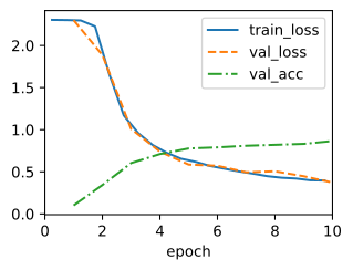
trainer = d2l.Trainer(max_epochs=10)
data = d2l.FashionMNIST(batch_size=128, resize=(224, 224))
with d2l.try_gpu():
    model = NiN(lr=0.05)
    trainer.fit(model, data)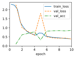
model = NiN(lr=0.05)
trainer = d2l.Trainer(max_epochs=10, num_gpus=1)
data = d2l.FashionMNIST(batch_size=128, resize=(224, 224))
trainer.fit(model, data)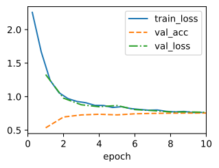
model = NiN(lr=0.05)
trainer = d2l.Trainer(max_epochs=10, num_gpus=1)
data = d2l.FashionMNIST(batch_size=128, resize=(224, 224))
trainer.fit(model, data)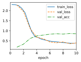
NiN has dramatically fewer parameters than AlexNet and VGG, primarily because it needs no giant fully connected layers. Instead, global average pooling replaces an expensive learned reduction with a simple average across locations. Under ideal translation equivariance, a translation merely permutes those locations, so the global average is invariant, although finite boundaries and strided stages make real networks only approximately shift-invariant. Two of NiN’s choices outlived it: \(1 \times 1\) convolution for channel mixing and global average pooling as the common classification head.
7.2.3 GoogLeNet: Multi-Branch Blocks and the Stem-Body-Head Pattern
In 2014, GoogLeNet won the ImageNet Challenge (Szegedy et al. 2015), using a structure that combined the strengths of NiN (Lin et al. 2013), repeated blocks (Simonyan and Zisserman 2015), and a cocktail of convolution kernels. It was arguably also the first network that exhibited a clear distinction among the stem (data ingest), body (data processing), and head (prediction) in a CNN. This design pattern has persisted ever since in the design of deep networks: the stem is the first two or three convolutions that operate on the image and extract its low-level features. This is followed by a body of convolutional blocks. Finally, the head maps the features obtained so far to the required classification, segmentation, detection, or tracking problem at hand.
GoogLeNet’s principal contribution was its multi-branch body. Instead of selecting one convolution size between \(1 \times 1\) and \(11 \times 11\), an Inception block applies several operations in parallel and concatenates their outputs. We present a simplified GoogLeNet; the original also used auxiliary classifiers at intermediate layers to stabilize training, which the implementations here omit.
7.2.3.1 The Inception Block
The basic convolutional block in GoogLeNet is called an Inception block, stemming from the meme “we need to go deeper” from the movie Inception.
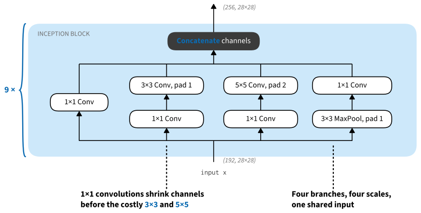
As depicted in Figure 7.2.3, the Inception block consists of four parallel branches. The first three branches use convolutional layers with window sizes of \(1\times 1\), \(3\times 3\), and \(5\times 5\) to extract information from different spatial sizes. The middle two branches also add a \(1\times 1\) convolution of the input to reduce the number of channels, reducing the model’s complexity. The fourth branch uses a \(3\times 3\) max-pooling layer, followed by a \(1\times 1\) convolutional layer to change the number of channels. The four branches all use appropriate padding to give the input and output the same height and width. Finally, the outputs along each branch are concatenated along the channel dimension and comprise the block’s output. The commonly tuned hyperparameters of the Inception block are the number of output channels per branch, i.e., how to allocate capacity among convolutions of different size.
class Inception(nn.Module):
    # c1--c4 are the number of output channels for each branch
    def __init__(self, c1, c2, c3, c4, **kwargs):
        super(Inception, self).__init__(**kwargs)
        # Branch 1
        self.b1_1 = nn.LazyConv2d(c1, kernel_size=1)
        # Branch 2
        self.b2_1 = nn.LazyConv2d(c2[0], kernel_size=1)
        self.b2_2 = nn.LazyConv2d(c2[1], kernel_size=3, padding=1)
        # Branch 3
        self.b3_1 = nn.LazyConv2d(c3[0], kernel_size=1)
        self.b3_2 = nn.LazyConv2d(c3[1], kernel_size=5, padding=2)
        # Branch 4
        self.b4_1 = nn.MaxPool2d(kernel_size=3, stride=1, padding=1)
        self.b4_2 = nn.LazyConv2d(c4, kernel_size=1)

    def forward(self, x):
        b1 = F.relu(self.b1_1(x))
        b2 = F.relu(self.b2_2(F.relu(self.b2_1(x))))
        b3 = F.relu(self.b3_2(F.relu(self.b3_1(x))))
        b4 = F.relu(self.b4_2(self.b4_1(x)))
        return torch.cat((b1, b2, b3, b4), dim=1)
class Inception(tf.keras.Model):
# c1--c4 are the number of output channels for each branch
def __init__(self, c1, c2, c3, c4):
super().__init__()
self.b1_1 = tf.keras.layers.Conv2D(c1, 1, activation='relu')
self.b2_1 = tf.keras.layers.Conv2D(c2[0], 1, activation='relu')
self.b2_2 = tf.keras.layers.Conv2D(c2[1], 3, padding='same',
activation='relu')
self.b3_1 = tf.keras.layers.Conv2D(c3[0], 1, activation='relu')
self.b3_2 = tf.keras.layers.Conv2D(c3[1], 5, padding='same',
activation='relu')
self.b4_1 = tf.keras.layers.MaxPool2D(3, 1, padding='same')
self.b4_2 = tf.keras.layers.Conv2D(c4, 1, activation='relu')
def call(self, x):
b1 = self.b1_1(x)
b2 = self.b2_2(self.b2_1(x))
b3 = self.b3_2(self.b3_1(x))
b4 = self.b4_2(self.b4_1(x))
return tf.keras.layers.Concatenate()([b1, b2, b3, b4])class Inception(nnx.Module):
def __init__(self, in_channels, c1, c2, c3, c4, rngs):
# Branch 1
self.b1_1 = nnx.Conv(in_channels, c1, kernel_size=(1, 1), rngs=rngs)
# Branch 2
self.b2_1 = nnx.Conv(in_channels, c2[0], kernel_size=(1, 1), rngs=rngs)
self.b2_2 = nnx.Conv(c2[0], c2[1], kernel_size=(3, 3),
padding='same', rngs=rngs)
# Branch 3
self.b3_1 = nnx.Conv(in_channels, c3[0], kernel_size=(1, 1), rngs=rngs)
self.b3_2 = nnx.Conv(c3[0], c3[1], kernel_size=(5, 5),
padding='same', rngs=rngs)
# Branch 4
self.b4_2 = nnx.Conv(in_channels, c4, kernel_size=(1, 1), rngs=rngs)
def __call__(self, x):
b1 = nnx.relu(self.b1_1(x))
b2 = nnx.relu(self.b2_2(nnx.relu(self.b2_1(x))))
b3 = nnx.relu(self.b3_2(nnx.relu(self.b3_1(x))))
pooled = nnx.max_pool(x, window_shape=(3, 3),
strides=(1, 1), padding='same')
b4 = nnx.relu(self.b4_2(pooled))
return jnp.concatenate((b1, b2, b3, b4), axis=-1)class Inception(nn.Block):
# c1--c4 are the number of output channels for each branch
def __init__(self, c1, c2, c3, c4):
super().__init__()
# Branch 1
self.b1_1 = nn.Conv2D(c1, kernel_size=1, activation='relu')
# Branch 2
self.b2_1 = nn.Conv2D(c2[0], kernel_size=1, activation='relu')
self.b2_2 = nn.Conv2D(c2[1], kernel_size=3, padding=1,
activation='relu')
# Branch 3
self.b3_1 = nn.Conv2D(c3[0], kernel_size=1, activation='relu')
self.b3_2 = nn.Conv2D(c3[1], kernel_size=5, padding=2,
activation='relu')
# Branch 4
self.b4_1 = nn.MaxPool2D(pool_size=3, strides=1, padding=1)
self.b4_2 = nn.Conv2D(c4, kernel_size=1, activation='relu')
def forward(self, x):
b1 = self.b1_1(x)
b2 = self.b2_2(self.b2_1(x))
b3 = self.b3_2(self.b3_1(x))
b4 = self.b4_2(self.b4_1(x))
return np.concatenate((b1, b2, b3, b4), axis=1)To see how the shapes work out, follow the first Inception block of the body on an ImageNet-sized input, where it receives 192 channels at \(28 \times 28\) resolution (the annotations in Figure 7.2.3). With branch outputs of \(c_1 = 64\), \(c_2 = (96, 128)\), \(c_3 = (16, 32)\), and \(c_4 = 32\), the block emits \(64+128+32+32 = 256\) channels at the same \(28 \times 28\) resolution: multi-branch blocks change the channel count, never the spatial size. The \(1 \times 1\) bottlenecks are what make the wide branches affordable. A direct \(5 \times 5\) convolution from 192 to 32 channels would need \(25 \cdot 192 \cdot 32 \approx 154\)k weights; squeezing to 16 channels first costs \(192 \cdot 16\) weights for the reduction plus \(25 \cdot 16 \cdot 32\) for the convolution, about 16k in total, a tenfold saving. This pattern of reducing channels before an expensive convolution recurs throughout the chapter.
Beyond economy, the combination of filters explores the image at a variety of spatial extents, so details of different sizes can be recognized by filters of the matching size, and the channel allocation decides how much capacity each scale receives.
7.2.3.2 Stem, Body, and Head
GoogLeNet arranges 9 Inception blocks into three groups of 2, 5, and 2, with max-pooling between the groups to reduce the resolution. The stem is AlexNet-like: a \(7 \times 7\) convolution with stride 2, a max-pooling step, then a \(1 \times 1\) and a \(3 \times 3\) convolution that raise the channel count to 192, and one more max-pooling step. The head is exactly NiN’s: global average pooling followed by a single fully connected layer.
The channel allocations inside the 9 blocks are data, not derivations. The paper picked them by hand, balancing the branches so that concatenation yields 256 up to 1024 channels as depth grows; the text itself offers no principle behind the exact ratios. At the time, automatic tools for design exploration were not yet available, and even input-shape inference, which we now take for granted, had to be done by the experimenter. We therefore store the allocation as a tuple of tuples, one entry per block, in the same architecture-as-data style as VGG’s arch:
arch = (((64, (96, 128), (16, 32), 32), (128, (128, 192), (32, 96), 64)),
        ((192, (96, 208), (16, 48), 64), (160, (112, 224), (24, 64), 64),
         (128, (128, 256), (24, 64), 64), (112, (144, 288), (32, 64), 64),
         (256, (160, 320), (32, 128), 128)),
        ((256, (160, 320), (32, 128), 128), (384, (192, 384), (48, 128), 128)))
Assembling the full network is now a matter of composing stem, body, and head.
class GoogleNet(d2l.Classifier):
    def __init__(self, lr=0.1, num_classes=10):
        super().__init__()
        self.save_hyperparameters()
        pool = lambda: nn.MaxPool2d(kernel_size=3, stride=2, padding=1)
        stem = nn.Sequential(
            nn.LazyConv2d(64, kernel_size=7, stride=2, padding=3), nn.ReLU(),
            pool(),
            nn.LazyConv2d(64, kernel_size=1), nn.ReLU(),
            nn.LazyConv2d(192, kernel_size=3, padding=1), nn.ReLU(), pool())
        body = [nn.Sequential(*[Inception(*c) for c in group])
                for group in arch]
        head = nn.Sequential(nn.AdaptiveAvgPool2d((1, 1)), nn.Flatten(),
                             nn.LazyLinear(num_classes))
        self.net = nn.Sequential(stem, body[0], pool(), body[1], pool(),
                                 body[2], head)
        self.net.apply(d2l.init_cnn)
class GoogleNet(d2l.Classifier):
def __init__(self, lr=0.1, num_classes=10):
super().__init__()
self.save_hyperparameters()
pool = lambda: tf.keras.layers.MaxPool2D(pool_size=3, strides=2,
padding='same')
stem = tf.keras.Sequential([
tf.keras.layers.Conv2D(64, 7, strides=2, padding='same',
activation='relu'), pool(),
tf.keras.layers.Conv2D(64, 1, activation='relu'),
tf.keras.layers.Conv2D(192, 3, padding='same', activation='relu'),
pool()])
body = [tf.keras.Sequential([Inception(*c) for c in group])
for group in arch]
head = tf.keras.Sequential([tf.keras.layers.GlobalAvgPool2D(),
tf.keras.layers.Dense(num_classes)])
self.net = tf.keras.Sequential([stem, body[0], pool(), body[1],
pool(), body[2], head])class GoogleNet(d2l.Classifier):
def __init__(self, lr=0.1, num_classes=10, rngs=None):
super().__init__()
self.save_hyperparameters(ignore=['rngs'])
rngs = nnx.Rngs(d2l.get_key()) if rngs is None else rngs
pool = lambda x: nnx.max_pool(
x, window_shape=(3, 3), strides=(2, 2), padding='same')
stem = nnx.Sequential(
nnx.Conv(1, 64, kernel_size=(7, 7), strides=(2, 2),
padding='same', rngs=rngs), nnx.relu, pool,
nnx.Conv(64, 64, kernel_size=(1, 1), rngs=rngs), nnx.relu,
nnx.Conv(64, 192, kernel_size=(3, 3), padding='same', rngs=rngs),
nnx.relu, pool)
body, in_channels = [], 192
for group in arch:
blocks = []
for c1, c2, c3, c4 in group:
blocks.append(Inception(
in_channels, c1, c2, c3, c4, rngs))
in_channels = c1 + c2[1] + c3[1] + c4
body.append(nnx.Sequential(*blocks))
head = nnx.Sequential(lambda x: x.mean(axis=(1, 2)),
nnx.Linear(in_channels, num_classes, rngs=rngs))
self.net = nnx.Sequential(stem, body[0], pool, body[1], pool,
body[2], head)class GoogleNet(d2l.Classifier):
def __init__(self, lr=0.1, num_classes=10):
super().__init__()
self.save_hyperparameters()
pool = lambda: nn.MaxPool2D(pool_size=3, strides=2, padding=1)
stem = nn.Sequential()
stem.add(nn.Conv2D(64, kernel_size=7, strides=2, padding=3,
activation='relu'), pool(),
nn.Conv2D(64, kernel_size=1, activation='relu'),
nn.Conv2D(192, kernel_size=3, padding=1, activation='relu'),
pool())
body = []
for group in arch:
blk = nn.Sequential()
blk.add(*[Inception(*c) for c in group])
body.append(blk)
self.net = nn.Sequential()
self.net.add(stem, body[0], pool(), body[1], pool(), body[2],
nn.GlobalAvgPool2D(), nn.Dense(num_classes))
self.net.initialize(init.Xavier())We check the shapes on a \(96 \times 96\) input, a resolution at which the network still works and the table stays compact. Resolution falls at the stem and at each pooling step between groups; the channel count grows after every group of Inception blocks, from 192 to 480 to 832 to 1024.
GoogleNet().layer_summary((1, 1, 96, 96))Sequential output shape: torch.Size([1, 192, 12, 12])
Sequential output shape: torch.Size([1, 480, 12, 12])
MaxPool2d output shape: torch.Size([1, 480, 6, 6])
Sequential output shape: torch.Size([1, 832, 6, 6])
MaxPool2d output shape: torch.Size([1, 832, 3, 3])
Sequential output shape: torch.Size([1, 1024, 3, 3])
Sequential output shape: torch.Size([1, 10])GoogleNet().layer_summary((1, 96, 96, 1))Sequential output shape: (1, 12, 12, 192)
Sequential output shape: (1, 12, 12, 480)
MaxPooling2D output shape: (1, 6, 6, 480)
Sequential output shape: (1, 6, 6, 832)
MaxPooling2D output shape: (1, 3, 3, 832)
Sequential output shape: (1, 3, 3, 1024)
Sequential output shape: (1, 10)GoogleNet().layer_summary((1, 96, 96, 1))Sequential output shape: (1, 12, 12, 192)
Sequential output shape: (1, 12, 12, 480)
function output shape: (1, 6, 6, 480)
Sequential output shape: (1, 6, 6, 832)
function output shape: (1, 3, 3, 832)
Sequential output shape: (1, 3, 3, 1024)
Sequential output shape: (1, 10)GoogleNet().layer_summary((1, 1, 96, 96))Sequential output shape: (1, 192, 12, 12)
Sequential output shape: (1, 480, 12, 12)
MaxPool2D output shape: (1, 480, 6, 6)
Sequential output shape: (1, 832, 6, 6)
MaxPool2D output shape: (1, 832, 3, 3)
Sequential output shape: (1, 1024, 3, 3)
GlobalAvgPool2D output shape: (1, 1024, 1, 1)
Dense output shape: (1, 10)Training follows the AlexNet and VGG procedure, so we do not repeat the run here. GoogLeNet uses about 7 million parameters, compared with VGG’s 138 million, while improving accuracy in the cited comparison. It therefore illustrates explicit trade-offs between evaluation cost and error, as well as manual experimentation with block-level hyperparameters. We revisit systematic network-structure exploration in Section 7.8.
GoogLeNet spawned a lineage: Inception-v2 and v3 (Szegedy et al. 2016) and Inception-v4 and Inception-ResNet (Szegedy et al. 2017) kept refining the branch mixtures. Direct descendants of Inception are less common in current backbone designs, and manually allocating heterogeneous branches has largely given way to more regular structures. Two Inception ideas persist in other forms. Grouped convolutions, as in ResNeXt (Section 7.4.5), are multi-branch blocks with all branches made identical, which removes the hand-tuning while keeping the cost savings. And RepVGG (Ding et al. 2021) uses parallel branches at training time only, fusing them into a single convolution for inference (Section 7.5).
7.2.4 Summary
Between 2013 and 2015, these architectures explored the design space opened by AlexNet. Although the original models are less common in current applications, their components continue to influence later networks.
| Idea | Introduced by | Current use |
|---|---|---|
| Repeated blocks, architecture as a tuple | VGG | many networks are specified stage by stage as block parameters |
| \(1 \times 1\) convolution | NiN | the channel-mixing layer in bottlenecks, ResNets, and transformers’ per-position MLPs |
| Global average pooling | NiN | a common classification head |
| Multi-branch blocks | GoogLeNet | grouped convolutions (ResNeXt) and train-time-only branches (RepVGG) |
The stem-body-head decomposition that GoogLeNet made explicit is now a common vocabulary for vision architectures, and we use it throughout the rest of the book. The next ingredient, which none of these networks had and all of their successors would adopt, is normalization.
7.2.5 Exercises
- Compared with AlexNet, VGG is much slower in terms of computation, and it also needs more GPU memory.
- Compare the number of parameters needed for AlexNet and VGG.
- Compare the number of floating point operations used in the convolutional layers and in the fully connected layers.
- How could you reduce the computational cost created by the fully connected layers?
- When displaying the dimensions associated with the various layers of the VGG network, we only see the information associated with eight blocks (plus some auxiliary transforms), even though the network has 11 layers. Where did the remaining three layers go?
- Use Table 1 in the VGG paper (Simonyan and Zisserman 2015) to construct other common models, such as VGG-16 or VGG-19.
- Upsampling the resolution in Fashion-MNIST eight-fold from \(28 \times 28\) to \(224 \times 224\) dimensions is very wasteful. Try modifying the network architecture and resolution conversion, e.g., to 56 or to 84 dimensions for its input instead. Can you do so without reducing the accuracy of the network? Consult the VGG paper (Simonyan and Zisserman 2015) for ideas on adding more nonlinearities prior to downsampling.
- Why are there two \(1\times 1\) convolutional layers per NiN block? Increase their number to three. Reduce their number to one. What changes?
- What happens if you replace NiN’s global average pooling by a fully connected layer (speed, accuracy, number of parameters)?
- What are possible problems with reducing the \(384 \times 5 \times 5\) representation to a \(10 \times 5 \times 5\) representation in one step, as the final NiN block does?
- Add a squeeze-and-excitation gate (Hu et al. 2018) to the Inception block: global-average-pool the block’s output to one value per channel, pass it through a two-layer MLP with a sigmoid at the end, and multiply the channels by the result. How many parameters does this add, and how does it change training on Fashion-MNIST?
- Replace the Inception block’s four branches with a single \(7 \times 7\) depthwise convolution followed by a \(1 \times 1\) convolution (Section 6.4.4). Compare the parameter count and the number of floating point operations with the original block at the same input and output sizes.
- What is the minimum image size needed for GoogLeNet to work? Can you design a variant that works on Fashion-MNIST’s native resolution of \(28 \times 28\) pixels? What would you need to change in the stem, the body, and the head?
- Compare the model parameter sizes of AlexNet, VGG, NiN, and GoogLeNet. How do the latter two architectures reduce the model parameter size so dramatically?