%matplotlib inline
from d2l import torch as d2l
import numpy as np
import torch
from torch import nn
from torch.func import functional_call, grad12.6 Learning at Test Time
The preceding sections introduced outer-product writes, several forms of decay, and delta-rule corrections. These updates can be interpreted as solving a regression problem at test time (Wang et al. 2025). As tokens arrive, the layer fits a small regressor to observed key–value pairs and answers each query by evaluating that fit.
This interpretation separates three design choices: how past pairs are weighted, the regressor’s function class, and the optimization method used for the inner fit. It also yields Longhorn, whose gate follows from an implicit update, and Titans, whose memory is a small neural network adapted during the forward pass. We conclude with drifting data, where emphasizing recent observations can reduce tracking error.
Prerequisites: attention as kernel regression (Section 10.1.3), the matrix-state family and its capacity law (Section 12.4), the delta rule (Section 12.5), and gradient descent with momentum and weight decay (Chapter 9). Every experiment in this section runs on a CPU.
We begin by learning the single parameter of the regression estimator introduced in Section 10.1.3.
%matplotlib inline
from d2l import jax as d2l
import jax
from jax import numpy as jnp
import numpy as np
12.6.1 Learning the Bandwidth
Recall where this book first met attention. In Section 10.1.3 we estimated a noisy function by Nadaraya–Watson regression (Nadaraya 1964; Watson 1964): keys were training inputs, values were their labels, and a Gaussian kernel turned each query into a weighted average of nearby values, Equation 10.1.3. Its bandwidth was not learned: we swept the kernel bandwidth \(\sigma\), by hand, and the section closed by asking what would happen if we learned it by gradient descent instead, warning that direct training on each point’s own target causes leakage. We now learn the bandwidth with a leave-one-out objective.
12.6.1.1 A Fixed Kernel, Revisited
We regenerate the dataset of Section 10.1.3, forty observations of \(y = 2\sin(x) + x\) under unit Gaussian noise, and the four-line estimator, which returns its attention-weight matrix alongside the fit. Sweeping the same three bandwidths and scoring against the noise-free function confirms what the fit curves showed there: the narrow kernel chases noise, the wide one oversmooths, and a mid-range bandwidth does best.
torch.manual_seed(0)
n = 40
x_train, _ = torch.sort(torch.rand(n) * 5)
y_train = 2 * torch.sin(x_train) + x_train + torch.randn(n)
x_val = torch.arange(0, 5, 0.1)
y_val = 2 * torch.sin(x_val) + x_val

def nadaraya_watson(x_train, y_train, x_val, sigma):
    dists = x_train[:, None] - x_val[None, :]
    k = torch.exp(-dists**2 / (2 * sigma**2))
    attention_w = k / k.sum(0)          # Normalize over keys for each query
    return y_train @ attention_w, attention_w

for sigma in (0.1, 0.5, 2.0):
    est, _ = nadaraya_watson(x_train, y_train, x_val, sigma)
    print(f'sigma = {sigma}: MSE against the noise-free function '
          f'{float(((est - y_val)**2).mean()):.3f}')
sigma = 0.1: MSE against the noise-free function 0.350
sigma = 0.5: MSE against the noise-free function 0.136
sigma = 2.0: MSE against the noise-free function 0.741key1, key2 = jax.random.split(jax.random.key(0))
n = 40
x_train = jnp.sort(jax.random.uniform(key1, (n,)) * 5)
y_train = 2 * jnp.sin(x_train) + x_train + jax.random.normal(key2, (n,))
x_val = jnp.arange(0, 5, 0.1)
y_val = 2 * jnp.sin(x_val) + x_val
def nadaraya_watson(x_train, y_train, x_val, sigma):
dists = x_train[:, None] - x_val[None, :]
k = jnp.exp(-dists**2 / (2 * sigma**2))
attention_w = k / k.sum(0) # Normalize over keys for each query
return y_train @ attention_w, attention_w
for sigma in (0.1, 0.5, 2.0):
est, _ = nadaraya_watson(x_train, y_train, x_val, sigma)
print(f'sigma = {sigma}: MSE against the noise-free function '
f'{float(((est - y_val)**2).mean()):.3f}')sigma = 0.1: MSE against the noise-free function 0.875
sigma = 0.5: MSE against the noise-free function 0.480
sigma = 2.0: MSE against the noise-free function 1.15512.6.1.2 Learning It, Without Cheating
To learn the bandwidth we make it a parameter. Writing \(w = 1/\sigma\) and folding it into the Gaussian kernel of Equation 10.1.3 gives a one-parameter regression model,
\[ f(x) = \sum_{i=1}^{n} \frac{\exp\big(-\tfrac{1}{2}\, ((x - x_i)\, w)^2\big)} {\sum_{j=1}^{n} \exp\big(-\tfrac{1}{2}\, ((x - x_j)\, w)^2\big)}\; y_i, \tag{12.6.1}\]
and the training loss is the squared error on the training points themselves. Each \(y_i\) then enters the computation of \(f(x_i)\). Driving \(w \to \infty\) shrinks the kernel until every training point attends only to itself, the training error drops to zero, and the estimator degenerates into a lookup table without constraining predictions between observations. Use a leave-one-out construction: when predicting at \(x_i\), the model may use every training pair except \((x_i, y_i)\). Below, each row of keys and values holds the other \(n-1\) points, built by masking the diagonal of a tiled copy of the data. Five epochs of plain gradient descent on the one scalar then suffice.
mask = ~torch.eye(n, dtype=torch.bool)
keys = x_train.repeat(n, 1)[mask].reshape(n, n - 1)    # Row i omits x_i
values = y_train.repeat(n, 1)[mask].reshape(n, n - 1)  # Row i omits y_i

w = torch.ones(1, requires_grad=True)
for epoch in range(5):
    attn = torch.softmax(-((x_train[:, None] - keys) * w)**2 / 2, dim=1)
    loss = ((attn * values).sum(1) - y_train).pow(2).mean()
    loss.backward()
    with torch.no_grad():
        w -= 0.5 * w.grad
        w.grad = None
    print(f'epoch {epoch + 1}: leave-one-out loss {float(loss.detach()):.3f}, '
          f'w = {float(w.detach()):.3f}')
w = w.detach()
assert float(w) > 1.0                   # Learning sharpened the kernel
print(f'learned bandwidth 1/w = {1 / float(w):.3f}')
epoch 1: leave-one-out loss 1.259, w = 1.268
epoch 2: leave-one-out loss 1.146, w = 1.428
epoch 3: leave-one-out loss 1.102, w = 1.545
epoch 4: leave-one-out loss 1.078, w = 1.637
epoch 5: leave-one-out loss 1.062, w = 1.716
learned bandwidth 1/w = 0.583mask = ~jnp.eye(n, dtype=bool)
keys = jnp.tile(x_train, (n, 1))[mask].reshape(n, n - 1) # Row i omits x_i
values = jnp.tile(y_train, (n, 1))[mask].reshape(n, n - 1) # Row i omits y_i
def loo_loss(w):
attn = jax.nn.softmax(-((x_train[:, None] - keys) * w)**2 / 2, axis=1)
return (((attn * values).sum(1) - y_train)**2).mean()
w = jnp.ones(())
for epoch in range(5):
loss, g = jax.value_and_grad(loo_loss)(w)
w -= 0.5 * g
print(f'epoch {epoch + 1}: leave-one-out loss {float(loss):.3f}, '
f'w = {float(w):.3f}')
assert float(w) > 1.0 # Learning sharpened the kernel
print(f'learned bandwidth 1/w = {1 / float(w):.3f}')epoch 1: leave-one-out loss 1.849, w = 1.266
epoch 2: leave-one-out loss 1.703, w = 1.541
epoch 3: leave-one-out loss 1.560, w = 1.781
epoch 4: leave-one-out loss 1.455, w = 1.975
epoch 5: leave-one-out loss 1.387, w = 2.132
learned bandwidth 1/w = 0.469The loss falls every epoch and \(w\) climbs well past its initialization at \(1\): gradient descent finds, in five steps, a bandwidth in the same region the hand sweep picked. The resulting fit and attention weights show the effect of this estimate.
12.6.1.3 Effect of the Learned Bandwidth
est_fixed, attn_fixed = nadaraya_watson(x_train, y_train, x_val, 1.0)
est_learned, attn_learned = nadaraya_watson(x_train, y_train, x_val,
                                            1 / float(w))
d2l.plot(x_val, [est_fixed, est_learned, y_val], 'x', 'y',
         legend=['sigma = 1 (before)', 'learned sigma (after)', 'truth'])
d2l.plt.plot(x_train, y_train, 'o', alpha=0.4);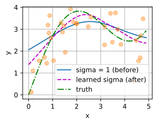
est_fixed, attn_fixed = nadaraya_watson(x_train, y_train, x_val, 1.0)
est_learned, attn_learned = nadaraya_watson(x_train, y_train, x_val,
                                            1 / float(w))
d2l.plot(x_val, [est_fixed, est_learned, y_val], 'x', 'y',
         legend=['sigma = 1 (before)', 'learned sigma (after)', 'truth'])
d2l.plt.plot(x_train, y_train, 'o', alpha=0.4);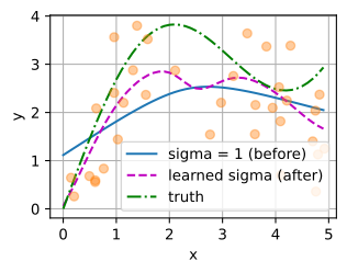
The learned fit bends where the function bends, recovering the rise and the crest that the \(\sigma = 1\) fit smooths away, while also following the noise a little more closely. The attention weights show the mechanism:
d2l.show_heatmaps(torch.stack([attn_fixed.T, attn_learned.T])[None],
                  xlabel='Training inputs (keys)',
                  ylabel='Validation inputs (queries)',
                  titles=['before (sigma = 1)', 'after (learned)'],
                  figsize=(7, 3))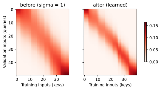
d2l.show_heatmaps(jnp.stack([attn_fixed.T, attn_learned.T])[None],
                  xlabel='Training inputs (keys)',
                  ylabel='Validation inputs (queries)',
                  titles=['before (sigma = 1)', 'after (learned)'],
                  figsize=(7, 3))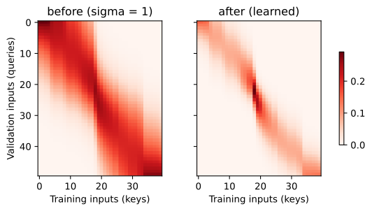
The region of large attention weights becomes sharper once the bandwidth is learned: each query concentrates on fewer, closer keys. After five epochs, the estimator has adapted its similarity scale using the data on which it will be queried. The same structure — a regression estimator fitted on the current sequence — describes the memories considered below.
12.6.2 Components of an Online Regressor
An autoregressive sequence layer admits the following general formulation. By time \(t\), the pairs \((\mathbf{k}_1, \mathbf{v}_1), \ldots, (\mathbf{k}_t, \mathbf{v}_t)\) and must answer the query \(\mathbf{q}_t\). Following Wang et al. (2025), treat this as two operations. Memorize: fit a regressor \(m_t\) from a function class \(\mathcal{M}\) to the observed pairs, weighting pair \(i\) by \(\gamma_i^{(t)} \ge 0\). Retrieve: evaluate it at the query.
\[ m_t \;=\; \mathop{\mathrm{argmin}}_{m \in \mathcal{M}}\; \frac{1}{2} \sum_{i \le t} \gamma_i^{(t)} \big\| \mathbf{v}_i - m(\mathbf{k}_i) \big\|^2, \qquad \mathbf{o}_t \;=\; m_t(\mathbf{q}_t). \tag{12.6.2}\]
The regression is solved afresh at every step, on the sequence being processed: it is learning at test time. This formulation involves two learning loops: an outer loop that trains the layer and an inner loop that runs within it. Section 12.6.2.1 defines this distinction precisely. A layer is then specified by three choices:
- The weights \(\gamma_i^{(t)}\): which past pairs count, and by how much.
- The function class \(\mathcal{M}\): what kinds of key-to-value association can be represented.
- The solver: how close to the argmin the layer actually gets, given that it must run inside a forward pass.
The models from the preceding three sections arise from different choices along these three axes in Equation 12.6.2.
Softmax attention is the Nadaraya–Watson estimator. Let \(\mathcal{M}\) be nonparametric: around each query, fit the best local constant, with pair \(i\) weighted by a kernel \(s(\mathbf{k}_i, \mathbf{q}_t)\). Setting the derivative of \(\sum_i s(\mathbf{k}_i, \mathbf{q}_t)\, \|\mathbf{v}_i - \mathbf{c}\|^2\) with respect to \(\mathbf{c}\) to zero gives \(\mathbf{o}_t = \sum_i s(\mathbf{k}_i, \mathbf{q}_t)\, \mathbf{v}_i / \sum_j s(\mathbf{k}_j, \mathbf{q}_t)\), which is Equation 10.1.3 verbatim. Choose the kernel \(s(\mathbf{k}, \mathbf{q}) = \exp(\mathbf{k}^\top \mathbf{q} / \sqrt{d})\) and this is exactly the softmax-attention readout of Chapter 10. Thus the kernel-regression interpretation used to introduce attention is an exact identity for this estimator. Softmax attention memorizes by keeping every pair and smoothing among them at query time; its “state” is the whole history, which is why its cache grows and a recurrence’s does not.
Linear attention is least squares with a term deleted. Let \(\mathcal{M}\) be linear maps \(m(\mathbf{k}) = \mathbf{S}^\top \mathbf{k}\) with uniform weights. Stack the keys as the rows of \(\mathbf{K}_t \in \mathbb{R}^{t \times d_k}\) and the values as the rows of \(\mathbf{V}_t \in \mathbb{R}^{t \times d_v}\). The minimizers of Equation 12.6.2 solve the normal equations \(\mathbf{K}_t^\top \mathbf{K}_t\, \mathbf{S} = \mathbf{K}_t^\top \mathbf{V}_t\), where the \(d_k \times d_k\) key covariance \(\mathbf{K}_t^\top \mathbf{K}_t\) has rank at most \(\min(t, d_k)\) — early in the sequence it is necessarily singular, so the well-posed statements come first: the minimum-norm solution through the pseudoinverse, or a ridge term,
\[ \mathbf{S}_t^\star = \mathbf{K}_t^{+} \mathbf{V}_t = \lim_{\lambda \downarrow 0}\, \big( \mathbf{K}_t^\top \mathbf{K}_t + \lambda \mathbf{I} \big)^{-1} \mathbf{K}_t^\top \mathbf{V}_t, \tag{12.6.3}\]
with the plain inverse \((\mathbf{K}_t^\top \mathbf{K}_t)^{-1} \mathbf{K}_t^\top \mathbf{V}_t\) legitimate once the covariance has full rank.
Now suppose the design is white: \(\mathbf{K}_t^\top \mathbf{K}_t \approx \mathbf{I}\), that is, the columns of \(\mathbf{K}_t\) are approximately orthonormal — the keys, in aggregate, have identity covariance. (This is a statement about the \(d_k\) columns of the design, not about the \(t\) stored keys being mutually orthogonal; for \(t > d_k\) the rows cannot all be orthonormal.) Then the inverse disappears: \(\mathbf{S}_t = \mathbf{K}_t^\top \mathbf{V}_t = \sum_{i \le t} \mathbf{k}_i \mathbf{v}_i^\top\), the running outer-product state of Equation 12.4.1 with identity transition. Linear attention is a memory that skips the covariance correction, and the price of the skipped term is the interference sum of Equation 12.4.2. Note the statistical character of that price: for random independent keys the cross-talk is zero in expectation, so the capacity ceiling measured in Section 12.4.1.1 is interference variance, not a systematic bias.
Decay is a choice of weights. Set \(\gamma_i^{(t)} = \prod_{j=i+1}^{t} \gamma_j\) with per-token discounts \(\gamma_j \in (0, 1]\) and keep everything else: Equation 12.6.2 becomes a weighted least-squares problem whose shortcut solution accumulates decayed outer products, which is the decay ladder of Section 12.4, from RetNet’s fixed scalar to the input-dependent gates of Mamba-2 and GLA. This gives the statistical interpretation stated there, subject to the same qualification as above: writing \(\boldsymbol{\Gamma}_t = \mathrm{diag}(\gamma_1^{(t)}, \ldots, \gamma_t^{(t)})\), the decayed state is the weighted cross-moment \(\mathbf{K}_t^\top \boldsymbol{\Gamma}_t \mathbf{V}_t\) — one half of the sufficient pair for weighted least squares. The exact minimizer also needs the weighted key covariance \(\mathbf{K}_t^\top \boldsymbol{\Gamma}_t \mathbf{K}_t\), and dropping it is the identical covariance-deletion shortcut. The gate determines how fast evidence expires. The final experiment identifies a setting in which this weighting improves estimation.
The delta rule is a solver. Keep the linear class and uniform weights, but instead of solving, take one stochastic-gradient step on the newest pair’s loss at each token. That step is the DeltaNet update; the identity was the substance of Section 12.5, one gradient step on \(\tfrac{1}{2}\|\mathbf{S}^\top \mathbf{k}_t - \mathbf{v}_t\|^2\) versus the Hebbian write’s blind accumulation, so we do not re-derive it here. In the recipe’s terms: DeltaNet differs from linear attention not in what it remembers but in how it fits, an online solver with a per-token step size \(\beta_t\) in place of no solver at all. Were the sequence to hold still, running the same gradient-descent solver for several passes would converge — from \(\mathbf{S} = \mathbf{0}\) and with a small enough step — to the minimum-norm least-squares memory Equation 12.6.3.
Table 12.6.1 assembles the corners, including the two rows this section still owes. The table is our reconstruction along the three axes of Wang et al. (2025); the delta-rule lineage traces back through the fast weight programmers (Schlag et al. 2021).
| model | weights \(\gamma_i^{(t)}\) | class \(\mathcal{M}\) | solver |
|---|---|---|---|
| softmax attention (Chapter 10) | kernel in the query, \(s(\mathbf{k}_i, \mathbf{q}_t)\) | locally constant (nonparametric) | exact: Nadaraya–Watson |
| linear attention | uniform | linear \(\mathbf{S}^\top \mathbf{k}\) | least squares minus \((\mathbf{K}^\top\mathbf{K})^{-1}\) |
| RetNet / GLA / Mamba-2 (Section 12.4) | geometric decay | linear | weighted least squares, same shortcut |
| DeltaNet (Section 12.5) | uniform, write gated by \(\beta_t\) | linear | one explicit SGD step per token |
| Longhorn | uniform, write gated by \(\beta_t\) | linear | one implicit (proximal) step per token |
| Titans | weight decay \(\alpha_t\) | deep MLP \(\mathcal{M}_{\mathbf{W}}\) | SGD with momentum |
| batch ridge (reference) | uniform | linear in features | exact solve |
One further solver maintains the exact solution of Equation 12.6.3 with a rank-one update per token: recursive least squares. It costs more state and more arithmetic than any row above, and the first exercise places it on the table.
12.6.2.1 Two Loops: What Learns When
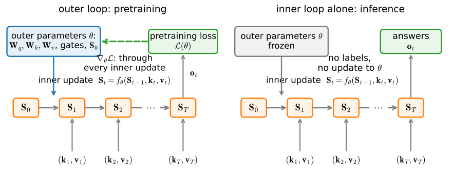
“Learning at test time” refers to two distinct adaptation schedules. Two different quantities adapt on different schedules (Figure 12.6.1).
The inner loop is the regression of Equation 12.6.2. Its variable is the layer’s state — the matrix \(\mathbf{S}_t\), or the memory weights \(\mathbf{W}_t\) of the Titans row — which starts fresh for every sequence, is updated token by token by the layer’s update rule, and is discarded when the sequence ends. This loop runs during every forward pass, in pretraining and at inference alike. At inference it is the only loop running: the state adapts online with no labels, because the regression targets are the values \(\mathbf{v}_t\) that the sequence itself supplies, and no parameter of the network changes.
The outer loop is ordinary pretraining. Its variables are the layer’s learned parameters \(\theta\): the projections that produce \(\mathbf{q}_t, \mathbf{k}_t, \mathbf{v}_t\), the networks that emit gates and step sizes (\(\beta_t\), \(\alpha_t\), and their kin), the state initialization, and any coefficients of the update rule itself. These receive gradients from the pretraining objective, and those gradients flow through the inner updates: a forward pass chains \(T\) state updates, and backpropagation differentiates the loss through every one of them. That is how a model learns to emit write strengths and decay rates that make its inner regressor fit well — when Section 12.5 trained delta-rule models end to end, the outer loop was shaping the inner one.
Thus, “no gradient at test time” refers only to the outer loop: at inference \(\theta\) is frozen and no pretraining objective exists, while the inner state keeps adapting. The distinction applies verbatim to every row of Table 12.6.1 — DeltaNet, Longhorn, and Titans differ in their inner update rules, and all three learn the coefficients of those rules in the outer loop. Readers who know meta-learning will recognize the two-level pattern: parameters optimized across sequences, state adapted within one.
12.6.2.2 Comparing Inner Solvers
If the rows of Table 12.6.1 really are one problem under different solvers, we should be able to hold the problem fixed and watch the solvers form a spectrum. We take one synthetic stream of eighty \((x, y)\) pairs from a noisy nonlinear function, and lift \(x\) into \(128\) random Fourier features \(\phi(x) = \sqrt{2/D}\,\cos(\mathbf{w} x + \mathbf{b})\) with random \(\mathbf{w}, \mathbf{b}\). Such features approximate a Gaussian kernel, so a linear memory over \(\phi\) is a kernel regressor, and the delta rule in \(\phi\)-space is its online form; this keeps every solver in the same function class while the problem stays one-dimensional enough to plot. Then we answer the same queries five ways: Nadaraya–Watson smoothing (softmax attention, no fitting at all), online gradient descent over the stream with one, five, and thirty passes (the delta rule, taken increasingly seriously as a solver), and the exact batch ridge solve.
A solver comparison is meaningful only when every solver optimizes the same objective. We therefore give each online step the same \(L2\) term the batch solve carries — a small per-step shrink of the weights, the decoupled decay of this chapter’s gated cells — so that online gradient descent and the batch solve are two solvers of one ridge problem, and “distance to the optimum” means distance to that shared problem’s minimizer. Nadaraya–Watson stays what it has always been: a different estimator family, with its own similarity and normalization, not an iteration count of this solver. Alongside test error we record each parametric fit’s value of the shared objective and its distance to the batch solution on the query grid, the direct measures of how far along the spectrum a solver sits.
torch.manual_seed(1)
n_ctx, num_feats, lam = 80, 128, 1e-2
x_ctx = torch.rand(n_ctx) * 6 - 3
y_ctx = torch.sin(1.5 * x_ctx) + 0.3 * x_ctx + 0.35 * torch.randn(n_ctx)
x_q = torch.linspace(-3, 3, 400)
y_q = torch.sin(1.5 * x_q) + 0.3 * x_q
w_feat = torch.randn(num_feats)
b_feat = torch.rand(num_feats) * 2 * torch.pi

def phi(x):                                  # Random Fourier features
    return torch.cos(x[:, None] * w_feat + b_feat) * (2 / num_feats)**0.5

def nw_attention(x_q, sigma=0.12):           # Softmax attention over the pairs
    logits = -(x_q[:, None] - x_ctx[None, :])**2 / (2 * sigma**2)
    return torch.softmax(logits, dim=1) @ y_ctx

feats = phi(x_ctx)

def objective(w):                            # The one shared ridge objective
    return float(0.5 * ((feats @ w - y_ctx)**2).sum() + 0.5 * lam * (w @ w))

def online_gd(passes, beta=0.06):            # Delta rule + per-step decay
    w_hat = torch.zeros(num_feats)
    for _ in range(passes):
        for f, v in zip(feats, y_ctx):       # SGD steps on the same objective
            w_hat = w_hat + beta * ((v - w_hat @ f) * f - lam / n_ctx * w_hat)
    return w_hat

w_batch = torch.linalg.solve(                # Exact minimizer, same objective
    feats.T @ feats + lam * torch.eye(num_feats), feats.T @ y_ctx)
f_batch = phi(x_q) @ w_batch

ws = {f'online GD, {p} pass' + ('es' if p > 1 else ''): online_gd(p)
      for p in (1, 5, 30)}
fits = {'Nadaraya-Watson': nw_attention(x_q)}
fits.update({name: phi(x_q) @ w for name, w in ws.items()})
fits['batch ridge'] = f_batch
objs = {name: objective(w) for name, w in ws.items()}
objs['batch ridge'] = objective(w_batch)
dist = {name: float(((f - f_batch)**2).mean()**0.5) for name, f in fits.items()}
print(f'{"solver":>22} {"test MSE":>9} {"objective":>10} {"dist to opt":>12}')
for name, f in fits.items():
    obj = f'{objs[name]:>10.3f}' if name in objs else f'{"--":>10}'
    print(f'{name:>22} {float(((f - y_q)**2).mean()):>9.3f} {obj} '
          f'{dist[name]:>12.3f}')
gd_names = [k for k in fits if k.startswith('online')]
gd, og = [dist[k] for k in gd_names], [objs[k] for k in gd_names]
assert gd[0] > gd[1] > gd[2]         # More solving moves closer to the optimum
assert og[0] > og[1] > og[2] > objs['batch ridge']   # On the SAME objective
assert float(((f_batch - y_q)**2).mean()) < \
    float(((fits['online GD, 1 pass'] - y_q)**2).mean())
solver test MSE objective dist to opt
Nadaraya-Watson 0.027 -- 0.135
online GD, 1 pass 0.070 8.916 0.277
online GD, 5 passes 0.027 6.238 0.100
online GD, 30 passes 0.022 6.134 0.077
batch ridge 0.010 5.860 0.000kc, kn, kw, kb = jax.random.split(jax.random.key(1), 4)
n_ctx, num_feats, lam = 80, 128, 1e-2
x_ctx = jax.random.uniform(kc, (n_ctx,)) * 6 - 3
y_ctx = (jnp.sin(1.5 * x_ctx) + 0.3 * x_ctx
+ 0.35 * jax.random.normal(kn, (n_ctx,)))
x_q = jnp.linspace(-3, 3, 400)
y_q = jnp.sin(1.5 * x_q) + 0.3 * x_q
w_feat = jax.random.normal(kw, (num_feats,))
b_feat = jax.random.uniform(kb, (num_feats,)) * 2 * jnp.pi
def phi(x): # Random Fourier features
return jnp.cos(x[:, None] * w_feat + b_feat) * (2 / num_feats)**0.5
def nw_attention(x_q, sigma=0.12): # Softmax attention over the pairs
logits = -(x_q[:, None] - x_ctx[None, :])**2 / (2 * sigma**2)
return jax.nn.softmax(logits, axis=1) @ y_ctx
feats = phi(x_ctx)
def objective(w): # The one shared ridge objective
return float(0.5 * ((feats @ w - y_ctx)**2).sum() + 0.5 * lam * (w @ w))
def online_gd(passes, beta=0.06): # Delta rule + per-step decay
def step(w_hat, fv):
f, v = fv # SGD steps on the same objective
return w_hat + beta * ((v - w_hat @ f) * f - lam / n_ctx * w_hat), None
w_hat = jnp.zeros(num_feats)
for _ in range(passes):
w_hat, _ = jax.lax.scan(step, w_hat, (feats, y_ctx))
return w_hat
w_batch = jnp.linalg.solve( # Exact minimizer, same objective
feats.T @ feats + lam * jnp.eye(num_feats), feats.T @ y_ctx)
f_batch = phi(x_q) @ w_batch
ws = {f'online GD, {p} pass' + ('es' if p > 1 else ''): online_gd(p)
for p in (1, 5, 30)}
fits = {'Nadaraya-Watson': nw_attention(x_q)}
fits.update({name: phi(x_q) @ w for name, w in ws.items()})
fits['batch ridge'] = f_batch
objs = {name: objective(w) for name, w in ws.items()}
objs['batch ridge'] = objective(w_batch)
dist = {name: float(((f - f_batch)**2).mean()**0.5) for name, f in fits.items()}
print(f'{"solver":>22} {"test MSE":>9} {"objective":>10} {"dist to opt":>12}')
for name, f in fits.items():
obj = f'{objs[name]:>10.3f}' if name in objs else f'{"--":>10}'
print(f'{name:>22} {float(((f - y_q)**2).mean()):>9.3f} {obj} '
f'{dist[name]:>12.3f}')
gd_names = [k for k in fits if k.startswith('online')]
gd, og = [dist[k] for k in gd_names], [objs[k] for k in gd_names]
assert gd[0] > gd[1] > gd[2] # More solving moves closer to the optimum
assert og[0] > og[1] > og[2] > objs['batch ridge'] # On the SAME objective
assert float(((f_batch - y_q)**2).mean()) < \
float(((fits['online GD, 1 pass'] - y_q)**2).mean()) solver test MSE objective dist to opt
Nadaraya-Watson 0.023 -- 0.114
online GD, 1 pass 0.151 9.372 0.372
online GD, 5 passes 0.022 5.108 0.128
online GD, 30 passes 0.008 4.542 0.031
batch ridge 0.010 4.487 0.000The results compare every parametric solver on the same objective. A single online pass visibly underfits, and a single pass is the budget an actual recurrent layer gets: its test error is several times the batch solve’s. More passes improve both solver columns monotonically — the shared objective falls toward the batch value, and the distance to the batch fit shrinks severalfold from one pass to thirty; the asserts pin these orderings rather than the digits, which move with the seed. One reading of the table deserves care: the “optimum” is the minimizer of the training objective, and on test error an unconverged iterate can land near it, in some of our runs slightly below it — stopping a solver early acts as a regularizer, so the objective column, not the test column, is what orders the solvers. Nadaraya–Watson sits off the parametric axis entirely, competitive in error yet fitting nothing, because it keeps all eighty pairs and smooths at query time. The fitted functions distinguish the three methods:
d2l.plot(x_q, [fits['Nadaraya-Watson'], fits['online GD, 1 pass'],
               fits['batch ridge'], y_q], 'x', 'y',
         legend=['Nadaraya-Watson', 'online GD, 1 pass', 'batch ridge',
                 'truth'])
d2l.plt.plot(x_ctx, y_ctx, 'o', alpha=0.3);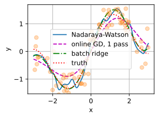
d2l.plot(x_q, [fits['Nadaraya-Watson'], fits['online GD, 1 pass'],
               fits['batch ridge'], y_q], 'x', 'y',
         legend=['Nadaraya-Watson', 'online GD, 1 pass', 'batch ridge',
                 'truth'])
d2l.plt.plot(x_ctx, y_ctx, 'o', alpha=0.3);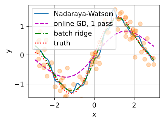
The kernel smoother is locally faithful and slightly ragged, the one-pass delta fit is smooth but shallow, still pulled toward zero where it has not finished learning, and the batch solve threads the noise. Every sequence layer in Table 12.6.1 is a point on this picture, chosen under a hard constraint the picture leaves out: the solver must run once per token, forward-only, in constant memory. This comparison leaves one question: can an affordable streaming update derive a form for the step size \(\beta_t\) from the optimization problem rather than using a designed gate?
12.6.3 Deriving the Gate: Longhorn
An implicit, or proximal, step provides such an update. It solves exactly for the state that balances proximity to the preceding state against fit to the newest pair. Longhorn (Liu et al. 2024) builds a state space model from precisely this update. Per output channel, with state \(\mathbf{s} \in \mathbb{R}^{d_k}\) (a column of the matrix state) and target \(v_t\),
\[ \mathbf{s}_t = \mathop{\mathrm{argmin}}_{\mathbf{s}}\; \big\| \mathbf{s} - \mathbf{s}_{t-1} \big\|^2 + \beta_t \big( \mathbf{s}^\top \mathbf{k}_t - v_t \big)^2 , \tag{12.6.4}\]
where \(\beta_t \ge 0\) sets how much the new evidence matters. The subproblem looks like it needs a matrix inverse per token. It does not.
Proposition. The unique minimizer of Equation 12.6.4 is
\[ \mathbf{s}_t = \big( \mathbf{I} - \Delta_t\, \mathbf{k}_t \mathbf{k}_t^\top \big)\, \mathbf{s}_{t-1} + \Delta_t\, v_t\, \mathbf{k}_t, \qquad \Delta_t = \frac{\beta_t}{1 + \beta_t\, \mathbf{k}_t^\top \mathbf{k}_t}. \tag{12.6.5}\]
Proof. The objective is strictly convex, so setting its gradient to zero characterizes the minimizer: \((\mathbf{I} + \beta_t \mathbf{k}_t \mathbf{k}_t^\top)\, \mathbf{s} = \mathbf{s}_{t-1} + \beta_t v_t \mathbf{k}_t\). By the Sherman–Morrison identity, \((\mathbf{I} + \beta_t \mathbf{k}_t \mathbf{k}_t^\top)^{-1} = \mathbf{I} - \Delta_t \mathbf{k}_t \mathbf{k}_t^\top\) with \(\Delta_t\) as stated; multiplying out and collecting terms gives Equation 12.6.5. \(\blacksquare\)
The update has the delta-rule shape of Section 12.5: it erases along the key and writes the correction. The algebra determines the functional form of its step size \(\Delta_t\). What remains learned is the coefficient that drives it — the model emits \(\beta_t\), and \(\Delta_t = \beta_t / (1 + \beta_t \mathbf{k}_t^\top \mathbf{k}_t)\) inherits that data dependence. The derived form also has a stability guarantee absent from an unconstrained explicit step. Since \(\Delta_t\, \mathbf{k}_t^\top \mathbf{k}_t = \beta_t \mathbf{k}_t^\top \mathbf{k}_t / (1 + \beta_t \mathbf{k}_t^\top \mathbf{k}_t) < 1\) for every \(\beta_t \ge 0\), the transition’s eigenvalue along the key stays in \((0, 1]\): the implicit step can approach a full overwrite as \(\beta_t \to \infty\) but can never overshoot into instability, no matter what the network emits for \(\beta_t\). The explicit delta rule buys stability by constraining its gate to a bounded range; the implicit rule is stable by construction. For small \(\beta_t\), \(\Delta_t \approx \beta_t\) and the two rules coincide. Compare the state transition of Section 12.3, whose input-dependent gate is a carefully chosen parameterization, a good design; here the form of the gate is a theorem, and only its coefficient is left to the model to learn. The distinction is worth having because derived updates generalize: change the objective and the machinery re-derives the architecture, which is exactly how the models of the next subsection arise. Longhorn’s authors report that this single change, the implicit step, matches or improves Mamba at equal size on language modeling, with better sample efficiency and extrapolation to contexts far past the training length (Liu et al. 2024).
The proposition is checkable in a few lines, and we should check it: we compare the closed form against a linear solve of the stationarity system over random instances, and against brute-force minimization of Equation 12.6.4 by gradient descent, which, run to convergence, must land on the same point the closed form reaches in one step.
def prox_step(s, k, v, beta):
    """Closed form for argmin ||s - s_prev||^2 + beta (s^T k - v)^2."""
    delta = beta / (1 + beta * (k @ k))
    return s - delta * (k @ s) * k + delta * v * k

torch.manual_seed(0)
dev_solve = dev_gd = 0.0
for trial in range(200):
    d = int(torch.randint(2, 16, (1,)))
    s_prev, k = torch.randn(d), torch.randn(d)
    v, beta = float(torch.randn(())), float(torch.rand(())) * 5 + 0.1
    s_cf = prox_step(s_prev, k, v, beta)
    lhs = torch.eye(d) + beta * torch.outer(k, k)   # Stationarity system
    s_exact = torch.linalg.solve(lhs, s_prev + beta * v * k)
    dev_solve = max(dev_solve, float((s_cf - s_exact).abs().max()))
    if trial < 5:                        # Gradient descent on the objective
        s = s_prev.clone().requires_grad_(True)
        lr = 0.5 / (1 + beta * float(k @ k))
        for _ in range(2000):
            obj = ((s - s_prev)**2).sum() + beta * (s @ k - v)**2
            g, = torch.autograd.grad(obj, s)
            s = (s - lr * g).detach().requires_grad_(True)
        dev_gd = max(dev_gd, float((s_cf - s.detach()).abs().max()))
print(f'closed form vs linear solve, 200 instances: {dev_solve:.2e}')
print(f'closed form vs gradient descent, 5 instances: {dev_gd:.2e}')
assert dev_solve < 1e-4 and dev_gd < 1e-4
closed form vs linear solve, 200 instances: 3.99e-06
closed form vs gradient descent, 5 instances: 1.34e-07def prox_step(s, k, v, beta):
"""Closed form for argmin ||s - s_prev||^2 + beta (s^T k - v)^2."""
delta = beta / (1 + beta * (k @ k))
return s - delta * (k @ s) * k + delta * v * k
dev_solve = dev_gd = 0.0
for trial in range(200):
kk = jax.random.split(jax.random.key(trial), 5)
d = int(jax.random.randint(kk[0], (), 2, 16))
s_prev = jax.random.normal(kk[1], (d,))
k = jax.random.normal(kk[2], (d,))
v = float(jax.random.normal(kk[3], ()))
beta = float(jax.random.uniform(kk[4], ())) * 5 + 0.1
s_cf = prox_step(s_prev, k, v, beta)
lhs = jnp.eye(d) + beta * jnp.outer(k, k) # Stationarity system
s_exact = jnp.linalg.solve(lhs, s_prev + beta * v * k)
dev_solve = max(dev_solve, float(jnp.abs(s_cf - s_exact).max()))
if trial < 5: # Gradient descent on the objective
def objective(s):
return ((s - s_prev)**2).sum() + beta * (s @ k - v)**2
lr = 0.5 / (1 + beta * float(k @ k))
def descend(s, _):
return s - lr * jax.grad(objective)(s), None
s, _ = jax.lax.scan(descend, s_prev, None, length=2000)
dev_gd = max(dev_gd, float(jnp.abs(s_cf - s).max()))
print(f'closed form vs linear solve, 200 instances: {dev_solve:.2e}')
print(f'closed form vs gradient descent, 5 instances: {dev_gd:.2e}')
assert dev_solve < 1e-4 and dev_gd < 1e-4closed form vs linear solve, 200 instances: 4.53e-06
closed form vs gradient descent, 5 instances: 2.38e-07Agreement to floating-point tolerance, across dimensions and gate strengths: two thousand explicit gradient steps arrive where the implicit step lands in closed form. In the full model, \(\beta_t\) (one per key channel) is emitted by a linear projection of the token exactly as DeltaNet emits its gate, and the layer trains in the same chunked parallel forms as the rest of the family (Section 12.4.3).
12.6.4 Deeper Memories: Titans
Two axes of the recipe remain unexplored. Every solver so far took plain gradient steps, and every memory so far was a linear map. Titans (Behrouz et al. 2025) pushes both at once: the memory is a module \(\mathcal{M}_{\mathbf{W}}\), possibly a small MLP, and its weights are trained during the forward pass by stochastic gradient descent with momentum and weight decay, the full optimizer toolkit of Chapter 9 running inside the sequence dimension. On the per-token recall loss \(\ell(\mathbf{W}; \mathbf{k}_t, \mathbf{v}_t) = \|\mathcal{M}_{\mathbf{W}}(\mathbf{k}_t) - \mathbf{v}_t\|^2\), the update keeps a velocity \(\mathbf{U}\) alongside the weights:
\[ \mathbf{U}_t = \eta_t\, \mathbf{U}_{t-1} - \theta_t\, \nabla_{\mathbf{W}}\, \ell(\mathbf{W}_{t-1}; \mathbf{k}_t, \mathbf{v}_t), \qquad \mathbf{W}_t = (1 - \alpha_t)\, \mathbf{W}_{t-1} + \mathbf{U}_t . \tag{12.6.6}\]
The paper interprets the three terms through their effects on adaptation. The gradient is momentary surprise: it is large exactly when the memory retrieves the wrong value for the current key. The momentum term \(\eta_t \mathbf{U}_{t-1}\) is past surprise, letting an unexpected event keep writing for several tokens after it occurs. And the weight decay \(\alpha_t\) is forgetting, the whole memory fading at a controllable, input-dependent rate. All three coefficients are emitted per token by the network. Two familiar corners sit inside Equation 12.6.6: with a linear memory, no momentum (\(\eta = 0\)), and no forgetting (\(\alpha = 0\)), the gradient identity of Section 12.5 turns the update into exactly the delta rule with \(\beta_t = 2\theta_t\); and \(\alpha_t\) alone reproduces the decay ladder acting on weights instead of a state matrix.
12.6.4.1 A Linear Memory, By Hand
For a linear memory the gradient is analytic, \(\nabla_{\mathbf{S}} \|\mathbf{S}^\top \mathbf{k} - \mathbf{v}\|^2 = 2\, \mathbf{k} (\mathbf{S}^\top \mathbf{k} - \mathbf{v})^\top\), so the whole Titans update runs in a dozen lines of NumPy with no autograd anywhere. This analytic update lets us test how momentum and forgetting affect the delta rule’s exact overwriting behavior, which keeps latest-value recall near \(1\). We repeat the overwrite protocol: write \(R\) values per key in shuffled order over orthonormal keys, then query every key for its latest value.
rng = np.random.default_rng(0)

def titans_linear(keys_seq, vals_seq, d=64, lr=0.5, eta=0.9, alpha=0.1):
    """Stream (key id, value id) pairs; return recall of each latest value."""
    key_mat = np.linalg.qr(rng.standard_normal((d, 8)))[0].T  # Orthonormal
    val_code = rng.standard_normal((32, d))
    val_code /= np.linalg.norm(val_code, axis=1, keepdims=True)
    S, U, latest = np.zeros((d, d)), np.zeros((d, d)), {}
    for i, j in zip(keys_seq, vals_seq):
        k, v = key_mat[i], val_code[j]
        latest[i] = j
        G = 2 * np.outer(k, S.T @ k - v)    # Analytic gradient: surprise
        U = eta * U - lr * G                # Momentum: past surprise
        S = (1 - alpha) * S + U             # Weight decay: forgetting
    hits = sum((val_code @ (S.T @ key_mat[i])).argmax() == j
               for i, j in latest.items())
    return hits / len(latest)

print(f'{"overwrites per key":>19} {"recall of latest":>17}')
recalls = []
for R in (1, 2, 4, 8):
    accs = []
    for _ in range(50):
        keys_seq = np.repeat(np.arange(8), R)
        vals_seq = rng.integers(0, 32, 8 * R)
        perm = rng.permutation(8 * R)
        accs.append(titans_linear(keys_seq[perm], vals_seq[perm]))
    recalls.append(np.mean(accs))
    print(f'{R:>19} {recalls[-1]:>17.3f}')
assert recalls[0] > 0.95 and recalls[-1] < 0.5
overwrites per key recall of latest
1 1.000
2 0.927
4 0.185
8 0.100rng = np.random.default_rng(0)
def titans_linear(keys_seq, vals_seq, d=64, lr=0.5, eta=0.9, alpha=0.1):
"""Stream (key id, value id) pairs; return recall of each latest value."""
key_mat = np.linalg.qr(rng.standard_normal((d, 8)))[0].T # Orthonormal
val_code = rng.standard_normal((32, d))
val_code /= np.linalg.norm(val_code, axis=1, keepdims=True)
S, U, latest = np.zeros((d, d)), np.zeros((d, d)), {}
for i, j in zip(keys_seq, vals_seq):
k, v = key_mat[i], val_code[j]
latest[i] = j
G = 2 * np.outer(k, S.T @ k - v) # Analytic gradient: surprise
U = eta * U - lr * G # Momentum: past surprise
S = (1 - alpha) * S + U # Weight decay: forgetting
hits = sum((val_code @ (S.T @ key_mat[i])).argmax() == j
for i, j in latest.items())
return hits / len(latest)
print(f'{"overwrites per key":>19} {"recall of latest":>17}')
recalls = []
for R in (1, 2, 4, 8):
accs = []
for _ in range(50):
keys_seq = np.repeat(np.arange(8), R)
vals_seq = rng.integers(0, 32, 8 * R)
perm = rng.permutation(8 * R)
accs.append(titans_linear(keys_seq[perm], vals_seq[perm]))
recalls.append(np.mean(accs))
print(f'{R:>19} {recalls[-1]:>17.3f}')
assert recalls[0] > 0.95 and recalls[-1] < 0.5 overwrites per key recall of latest
1 1.000
2 0.927
4 0.185
8 0.100At one write per key, recall is perfect; at two it is still high; by four and eight overwrites it collapses toward chance (chance is about \(0.03\) here). Momentum has made the memory a softer overwriter than the pure delta rule, and the mechanism is visible in Equation 12.6.6: the surprise from an earlier binding persists in \(\mathbf{U}\) and keeps writing the superseded value for several more steps, while \(\alpha\) erodes keys that were never touched. The result isolates the bias introduced by momentum. Momentum smooths the fit across tokens, which is the wrong bias when the stream rebinds keys adversarially and a useful one when successive tokens carry consistent evidence, precisely the regime that this section’s closing experiment returns to, as does one of the exercises.
12.6.4.2 A Deep Memory via Autograd
Why make the memory deep? Because the function class \(\mathcal{M}\) is a choice, and the linear choice has a hard ceiling: the capacity law of Section 12.4.1.1 is a statement about linear maps, at most \(d_k\) associations retrievable without interference, however clever the solver. An MLP memory is not superposition-bound in the same way, and Titans reports that deeper memories keep improving language modeling at scale (Behrouz et al. 2025). The update Equation 12.6.6 does not care what \(\mathcal{M}_{\mathbf{W}}\) is; only the gradient call changes, and for that we have autograd. Two functional gradient interfaces fit the task exactly, torch.func.grad and jax.grad, since the memory’s weights are data now, one set per sequence, not module state.
We initialize the output layer to zero, so the memory starts empty (every key retrieves \(\mathbf{0}\), just as \(\mathbf{S} = \mathbf{0}\) does), then stream \(64\) tokens in which each of \(16\) associations recurs four times in shuffled order, as facts recur in a document. Each token applies three operations: compute the gradient, update the velocity, and update the memory.
torch.manual_seed(0)
d_mem, h_mem, num_pairs = 32, 128, 16
k_pairs = nn.functional.normalize(torch.randn(num_pairs, d_mem), dim=-1)
v_pairs = nn.functional.normalize(torch.randn(num_pairs, d_mem), dim=-1)
order = torch.randperm(num_pairs * 4) % num_pairs   # Each pair recurs 4x

memory = nn.Sequential(nn.Linear(d_mem, h_mem), nn.GELU(),
                       nn.Linear(h_mem, d_mem))
with torch.no_grad():
    memory[0].weight.normal_(0, 1.0)    # Unit-variance hidden units
    memory[0].bias.zero_()
    memory[2].weight.zero_()            # Start empty: retrieve 0 everywhere
    memory[2].bias.zero_()

def recall_loss(params, k, v):
    return ((functional_call(memory, params, (k[None],))[0] - v)**2).sum()
grad_fn = grad(recall_loss)

def retrieval_mse(params):
    with torch.no_grad():
        pred = functional_call(memory, params, (k_pairs,))
    return float(((pred - v_pairs)**2).mean())

params = {name: p.detach().clone() for name, p in memory.named_parameters()}
velocity = {name: torch.zeros_like(p) for name, p in params.items()}
before = retrieval_mse(params)
theta, eta = 0.005, 0.5
for t in order.tolist():
    g = grad_fn(params, k_pairs[t], v_pairs[t])     # Surprise
    for name in params:
        velocity[name] = eta * velocity[name] - theta * g[name]
        params[name] = params[name] + velocity[name]
after = retrieval_mse(params)
print(f'retrieval MSE: empty memory {before:.4f} -> after the stream '
      f'{after:.4f}')
assert after < before / 5
retrieval MSE: empty memory 0.0312 -> after the stream 0.0023d_mem, h_mem, num_pairs = 32, 128, 16
ks = jax.random.split(jax.random.key(3), 4)
k_pairs = jax.random.normal(ks[0], (num_pairs, d_mem))
k_pairs /= jnp.linalg.norm(k_pairs, axis=1, keepdims=True)
v_pairs = jax.random.normal(ks[1], (num_pairs, d_mem))
v_pairs /= jnp.linalg.norm(v_pairs, axis=1, keepdims=True)
order = jax.random.permutation(ks[2], jnp.tile(jnp.arange(num_pairs), 4))
params = {'W1': jax.random.normal(ks[3], (d_mem, h_mem)), # Unit-var hidden
'b1': jnp.zeros(h_mem),
'W2': jnp.zeros((h_mem, d_mem)), # Start empty: retrieve 0
'b2': jnp.zeros(d_mem)}
def memory(params, k):
hidden = jax.nn.gelu(k @ params['W1'] + params['b1'])
return hidden @ params['W2'] + params['b2']
def recall_loss(params, k, v):
return ((memory(params, k) - v)**2).sum()
grad_fn = jax.grad(recall_loss)
def retrieval_mse(params):
return float(((memory(params, k_pairs) - v_pairs)**2).mean())
before = retrieval_mse(params)
theta, eta = 0.005, 0.5
def write(carry, t):
params, velocity = carry
g = grad_fn(params, k_pairs[t], v_pairs[t]) # Surprise
velocity = jax.tree.map(lambda u, gg: eta * u - theta * gg, velocity, g)
params = jax.tree.map(lambda p, u: p + u, params, velocity)
return (params, velocity), None
velocity = jax.tree.map(jnp.zeros_like, params)
(params, _), _ = jax.lax.scan(write, (params, velocity), order)
after = retrieval_mse(params)
print(f'retrieval MSE: empty memory {before:.4f} -> after the stream '
f'{after:.4f}')
assert after < before / 5retrieval MSE: empty memory 0.0312 -> after the stream 0.0013Retrieval error falls by more than an order of magnitude from the empty-memory baseline, on a CPU, in well under a second: the inner loop of Section 12.6.2.1 ran alone, a fresh neural memory adapting online inside what is conceptually a single forward pass over \(64\) tokens. Keep the two loops straight here: in this standalone demo every outer quantity — the coefficients \(\theta, \eta\), the initialization — was set by hand, whereas in the full Titans model those are outer-loop parameters, learned during pretraining together with the projections that produce keys and values, so the model learns how its memory should adapt. In the full architecture this neural memory is one branch of a layer; Titans studies three ways of wiring it to attention, as context (retrieved memories are prepended to the window that attention reads, MAC), as a gate (the memory branch and a sliding-window-attention branch are fused multiplicatively, MAG), or as a layer (memory feeding attention in series, MAL), with the context wiring strongest in their long-context evaluations. Wiring memories to attention at the layer scale is exactly the hybrid question this chapter closes with. Beyond Titans lies an active line of work on richer test-time objectives and solvers, from TTT’s mini-batch inner loop (Sun et al. 2024) onward; the chapter’s Resources section maps it, and this book stops at the recipe.
12.6.5 Tracking Distribution Drift
The remaining statistical question concerns the weights \(\gamma_i^{(t)}\). The preceding measurements treated the stream as stationary, the capacity of Section 12.4.1.1 and the spectrum above alike. For a fixed target, a linear model that contains it, and constant parameters, uniform weights are then the efficient choice: every observation is equally informative about the same quantity. Decay becomes useful when the regression target changes over time. A forecasting example provides a statistical explanation for gating, decay, and test-time adaptation.
Take a streaming linear regression whose ground truth drifts: targets \(v_t = \mathbf{w}^{*\top}_t \mathbf{k}_t + \epsilon_t\), where \(\mathbf{w}^*_t\) takes a small random step on the unit sphere at every time step. We track it three ways, all rows of Table 12.6.1. First, uniform least squares: the exact solver over all history, our batch-ridge optimum streamed via its sufficient statistics. Second, decayed least squares: the same exact solver, but the statistics are discounted by \(\gamma = 0.95\) per step, weighted least squares, the statistical content of the decay ladder. Third, the implicit step of Equation 12.6.5 with fixed \(\beta\): no matrix solve at all, one \(\mathcal{O}(d)\) update per token, the derived gate doing its work.
rng = np.random.default_rng(2)
d, T, gamma, beta = 8, 2000, 0.95, 1.0
w_star = rng.standard_normal(d)
w_star /= np.linalg.norm(w_star)
stats_u = [np.zeros((d, d)), np.zeros(d)]   # Uniform sufficient statistics
stats_g = [np.zeros((d, d)), np.zeros(d)]   # Decayed sufficient statistics
s = np.zeros(d)                             # Implicit-step state
errs = {'uniform LS': [], 'decayed LS': [], 'implicit step': []}
ridge = 1e-6 * np.eye(d)
for t in range(T):
    w_star = w_star + 0.03 * rng.standard_normal(d)   # The world drifts
    w_star /= np.linalg.norm(w_star)
    k = rng.standard_normal(d) / np.sqrt(d)
    v = w_star @ k + 0.1 * rng.standard_normal()
    stats_u[0] += np.outer(k, k)
    stats_u[1] += v * k
    stats_g[0] = gamma * stats_g[0] + np.outer(k, k)
    stats_g[1] = gamma * stats_g[1] + v * k
    s = s + beta / (1 + beta * k @ k) * (v - s @ k) * k   # Derived gate
    for name, w_hat in (
            ('uniform LS', np.linalg.solve(stats_u[0] + ridge, stats_u[1])),
            ('decayed LS', np.linalg.solve(stats_g[0] + ridge, stats_g[1])),
            ('implicit step', s)):
        errs[name].append(np.linalg.norm(w_hat - w_star))

def smooth(e):
    return np.convolve(np.array(e), np.ones(50) / 50, mode='valid')

curves = [smooth(e) for e in errs.values()]
d2l.plot(np.arange(len(curves[0])), curves, 'step', 'tracking error',
         legend=list(errs))
tails = {name: float(np.mean(e[-500:])) for name, e in errs.items()}
print('mean error over the last 500 steps:',
      {name: round(v, 2) for name, v in tails.items()})
assert tails['uniform LS'] > 2 * tails['decayed LS']
assert tails['uniform LS'] > 2 * tails['implicit step']
mean error over the last 500 steps: {'uniform LS': 0.99, 'decayed LS': 0.29, 'implicit step': 0.3}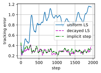
rng = np.random.default_rng(2)
d, T, gamma, beta = 8, 2000, 0.95, 1.0
w_star = rng.standard_normal(d)
w_star /= np.linalg.norm(w_star)
stats_u = [np.zeros((d, d)), np.zeros(d)]   # Uniform sufficient statistics
stats_g = [np.zeros((d, d)), np.zeros(d)]   # Decayed sufficient statistics
s = np.zeros(d)                             # Implicit-step state
errs = {'uniform LS': [], 'decayed LS': [], 'implicit step': []}
ridge = 1e-6 * np.eye(d)
for t in range(T):
    w_star = w_star + 0.03 * rng.standard_normal(d)   # The world drifts
    w_star /= np.linalg.norm(w_star)
    k = rng.standard_normal(d) / np.sqrt(d)
    v = w_star @ k + 0.1 * rng.standard_normal()
    stats_u[0] += np.outer(k, k)
    stats_u[1] += v * k
    stats_g[0] = gamma * stats_g[0] + np.outer(k, k)
    stats_g[1] = gamma * stats_g[1] + v * k
    s = s + beta / (1 + beta * k @ k) * (v - s @ k) * k   # Derived gate
    for name, w_hat in (
            ('uniform LS', np.linalg.solve(stats_u[0] + ridge, stats_u[1])),
            ('decayed LS', np.linalg.solve(stats_g[0] + ridge, stats_g[1])),
            ('implicit step', s)):
        errs[name].append(np.linalg.norm(w_hat - w_star))

def smooth(e):
    return np.convolve(np.array(e), np.ones(50) / 50, mode='valid')

curves = [smooth(e) for e in errs.values()]
d2l.plot(np.arange(len(curves[0])), curves, 'step', 'tracking error',
         legend=list(errs))
tails = {name: float(np.mean(e[-500:])) for name, e in errs.items()}
print('mean error over the last 500 steps:',
      {name: round(v, 2) for name, v in tails.items()})
assert tails['uniform LS'] > 2 * tails['decayed LS']
assert tails['uniform LS'] > 2 * tails['implicit step']
mean error over the last 500 steps: {'uniform LS': 0.99, 'decayed LS': 0.29, 'implicit step': 0.3}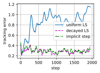
The curves separate as the regression view predicts. For the first few dozen steps the three trackers are indistinguishable, since with little drift accumulated, all evidence is informative. Uniform least squares then becomes stale: its error rises steadily and ends several times above the other methods because old observations retain full weight after the target has changed. The solver remains exact and the function class contains the truth; only the observation weights are misspecified. Decayed least squares is the same solver with expiring evidence, and it tracks the drift indefinitely; the implicit step tracks nearly as well with no solve, no matrix, and a step size \(\Delta_t\) it derived for itself.
A sequence model predicting a nonstationary stream, such as a market or conversation, must regress recent structure onto the present without giving equal weight to observations from an obsolete regime. Decay encodes an assumption about how fast the process changes. In the cell above, that assumption was fixed rather than learned from the data: we fixed \(\gamma = 0.95\) and \(\beta = 1\) by hand, and a differently paced drift would want different values. The trained models of this chapter emit these coefficients per token — the input-dependent gates of Section 12.4, the write strengths of Section 12.5, the surprise-driven learning rates of Titans — which is what lets the data set its own discount, a capability this fixed-coefficient cell motivates rather than demonstrates. The conclusion that the experiment does support is the scoped one: forgetting reduces tracking error under drift, at the price of statistical efficiency on stationary stretches.
Experimental scope. The bandwidth, spectrum, Longhorn, Titans, and drift cells are identity checks and mechanism illustrations on synthetic streams: they verify derivations (the closed-form implicit step), exhibit solver behavior (underfit approaching the shared optimum; momentum softening overwrites; staleness under drift), and settle nothing about language modeling at scale. The production-scale claims — which update rules ship, at what quality — rest on the cited papers.
12.6.6 Summary
This section described several architectures with one regression problem. A sequence-mixing layer maintains an associative memory by solving the weighted regression Equation 12.6.2 at test time and answers queries by evaluating the fit; a layer is fixed by its weights, its function class, and its solver. Under that reading, softmax attention is the Nadaraya–Watson estimator, the identity closing the loop opened when this book introduced attention through kernel regression, and our opening experiment learned the one parameter that classical estimator has, its bandwidth, by leave-one-out gradient descent, sharpening its attention weights. Linear attention is least squares with the key covariance deleted, its capacity ceiling the interference of that deletion; decay keeps the weighted cross-moment of a weighted least-squares problem; the delta rule is one explicit gradient step, and the measured spectrum — every parametric solver on one shared ridge objective — confirms that more solving lands closer to that objective’s optimum. Throughout, the two-loop distinction of Section 12.6.2.1 governs what “learning at test time” means: the inner state adapts online in every forward pass, while the outer parameters (the projections, gate networks, and initializations) receive gradients only during pretraining, flowing through the chain of inner updates. The two new models were both derived: the form of Longhorn’s gate \(\Delta_t\) is the closed-form implicit step of a per-token objective, its coefficient \(\beta_t\) still learned, stable by construction where explicit steps must be clamped, and Titans adapts a deep memory online inside the forward pass with momentum as persisting surprise and weight decay as forgetting, a softer overwriter than the delta rule but an expressively deeper one. Against a drifting target, exact uniform regression goes stale while decayed and implicit solvers track, which is the statistical reason forgetting exists. None of these fixed-size memories can recall an arbitrary needle from an arbitrarily long haystack, which sets up the chapter’s closing question in Section 12.7: how much genuine attention a model must keep.
12.6.7 Exercises
- [short-code] Recursive least squares joins the table. The exact solution Equation 12.6.3 can be maintained online: with \(\mathbf{P}_t = (\mathbf{K}_t^\top \mathbf{K}_t + \lambda \mathbf{I})^{-1}\), use the Sherman–Morrison identity to derive the rank-one update of \(\mathbf{P}_t\) and of the memory when \((\mathbf{k}_t, \mathbf{v}_t)\) arrives. Implement it on the spectrum problem of Section 12.6.2.2 and verify that after one pass it matches the batch ridge fit to numerical precision. What does it cost per token in memory and arithmetic compared with the delta rule, and where does it sit in Table 12.6.1?
- [conceptual] Derive Equation 12.6.5 yourself: write the stationarity condition of Equation 12.6.4, apply Sherman–Morrison, and check the two limits \(\beta_t \to 0\) (explicit gradient step) and \(\beta_t \to \infty\) (exact interpolation of the newest pair). For unit-norm keys, what range does \(\Delta_t\) cover?
- [short-code] In Section 12.6.1, remove the leave-one-out masking and train \(w\) on the plain training error. Report where \(w\) goes and what the fit looks like, then explain why a causal memory, which can only regress pairs from strictly earlier steps, gets the exclusion for free.
- [conceptual] With unit-norm keys and queries, expand \(\|\mathbf{q} - \mathbf{k}\|^2\) to show the Gaussian kernel of Equation 12.6.1 equals \(\exp(\mathbf{q}^\top \mathbf{k}\, w^2)\) up to query-independent factors, so the learned bandwidth is a learned softmax temperature. Which normalization schemes in modern attention stacks make this correspondence exact?
- [short-code] On the drifting stream of Section 12.6.5, add momentum to the implicit tracker as in Equation 12.6.6. Sweep \(\eta \in \{0, 0.5, 0.9\}\) under (a) the random-walk drift above and (b) a consistent drift that rotates \(\mathbf{w}^*_t\) steadily in a fixed plane. When does past surprise help, and why?
- [short-code] In the spectrum experiment, the thirty-pass fit’s distance to the batch solution is small but not zero. Explain the two remaining causes (the fixed step size \(\beta\) and the finite number of passes over one fixed ordering of the stream) and check both by shrinking \(\beta\) while increasing the passes. Then remove the \(L2\) term from the online steps only and rerun: the distance now stalls at a floor that no number of passes removes, because the online and batch solvers no longer share an objective. Which solution does plain online gradient descent from \(\mathbf{w} = \mathbf{0}\) approach instead?