%matplotlib inline
from d2l import torch as d2l
import torch
from torch import nn10.3 Multi-Head and Cross-Attention
Scaled dot-product attention assigns each query one distribution over the keys and returns one weighted average of the values. A single average cannot preserve several independently requested values. We demonstrate this limitation on a task for which any single head loses half of the target variance. Multi-head attention (Vaswani et al. 2017) computes several projected attention outputs and combines them linearly. With the usual choice of head dimensions, this changes the representation without changing the leading parameter or FLOP counts. We then distinguish self-attention and cross-attention as two input configurations of the same operation.
%matplotlib inline
from d2l import jax as d2l
from flax import nnx
import jax
from jax import numpy as jnp
10.3.1 A One-Mixture Bottleneck with Position-Only Keys
Consider a task that exposes this limitation. Two source positions hold value vectors \(\mathbf{v}_1, \mathbf{v}_2 \in \mathbb{R}^d\), drawn independently at random for every example; their keys mark only the positions, not the content. A query must report both values: the target is the concatenation \(\mathbf{t} = [\mathbf{v}_1; \mathbf{v}_2] \in \mathbb{R}^{2d}\). Think of a pronoun that must simultaneously retrieve its antecedent and its governing verb.
A single head can only produce, for this query, softmax weights \((\alpha_1, \alpha_2)\) with \(\alpha_1 + \alpha_2 = 1\), the mixture \(\mathbf{m} = \alpha_1 \mathbf{v}_1 + \alpha_2 \mathbf{v}_2\), and then a linear readout \(\mathbf{W}_o \mathbf{m}\). Since the keys are fixed position markers, the weights cannot depend on the values: whatever the head learns, it applies the same mixture to every example. How well can it do?
Proposition. Consider one attention layer with two fixed, position-only keys, independent isotropic Gaussian values, no residual path, and a linear readout. For the copy-both task, the best achievable relative squared error of a single head is \(1/2\) for every softmax pair \((\alpha_1,\alpha_2)\).
Proof. Given the mixture \(\mathbf{m} = \alpha_1 \mathbf{v}_1 + \alpha_2 \mathbf{v}_2\), the best estimate of \(\mathbf{v}_1\) is the conditional mean \(\mathbb{E}[\mathbf{v}_1 \mid \mathbf{m}] = \tfrac{\alpha_1}{\alpha_1^2 + \alpha_2^2}\, \mathbf{m}\), which is linear, so a linear readout attains it. Its per-dimension error variance is \(1 - \tfrac{\alpha_1^2}{\alpha_1^2 + \alpha_2^2} = \tfrac{\alpha_2^2}{\alpha_1^2 + \alpha_2^2}\); the error for \(\mathbf{v}_2\) is \(\tfrac{\alpha_1^2}{\alpha_1^2 + \alpha_2^2}\). The two errors sum to exactly \(1\) per dimension, while the target’s total variance is \(2\) per dimension. Thus the relative squared error is \(1/2\) regardless of how the head splits its attention. \(\blacksquare\)
Changing the softmax weights cannot remove the error because one head supplies the readout with only a single mixture of the two values. The following experiment verifies the bound.
torch.manual_seed(0)
N, d = 10000, 16
V1, V2 = torch.randn(N, d), torch.randn(N, d)
target = torch.cat([V1, V2], dim=1)

def readout_error(M, target):
    """Best linear readout of target from M, relative error."""
    W = torch.linalg.lstsq(M, target).solution
    return ((M @ W - target).norm() / target.norm()).item()

for a in (0.5, 0.7, 0.9, 1.0):
    M = a * V1 + (1 - a) * V2
    print(f'single head, weights ({a:.1f}, {1 - a:.1f}): '
          f'relative error {readout_error(M, target):.3f}')
print(f'theory: sqrt(1/2) = {0.5 ** 0.5:.3f}')
single head, weights (0.5, 0.5): relative error 0.706
single head, weights (0.7, 0.3): relative error 0.706
single head, weights (0.9, 0.1): relative error 0.706
single head, weights (1.0, 0.0): relative error 0.707
theory: sqrt(1/2) = 0.707N, d = 10000, 16
key1, key2 = jax.random.split(jax.random.key(0))
V1, V2 = jax.random.normal(key1, (N, d)), jax.random.normal(key2, (N, d))
target = jnp.concatenate([V1, V2], axis=1)
def readout_error(M, target):
"""Best linear readout of target from M, relative error."""
W = jnp.linalg.lstsq(M, target)[0]
return float(jnp.linalg.norm(M @ W - target) / jnp.linalg.norm(target))
for a in (0.5, 0.7, 0.9, 1.0):
M = a * V1 + (1 - a) * V2
print(f'single head, weights ({a:.1f}, {1 - a:.1f}): '
f'relative error {readout_error(M, target):.3f}')
print(f'theory: sqrt(1/2) = {0.5 ** 0.5:.3f}')single head, weights (0.5, 0.5): relative error 0.706
single head, weights (0.7, 0.3): relative error 0.706
single head, weights (0.9, 0.1): relative error 0.705
single head, weights (1.0, 0.0): relative error 0.705
theory: sqrt(1/2) = 0.707The error sits at \(\sqrt{1/2} \approx 0.707\) across the whole range, exactly as computed. Now give the model a second head: two sets of attention weights, their outputs concatenated before the readout.
for a in (1.0, 0.88):
    M2 = torch.cat([a * V1 + (1 - a) * V2,
                    (1 - a) * V1 + a * V2], dim=1)
    print(f'two heads, weights ({a:.2f}, {1 - a:.2f}) and '
          f'({1 - a:.2f}, {a:.2f}): '
          f'relative error {readout_error(M2, target):.1e}')
two heads, weights (1.00, 0.00) and (0.00, 1.00): relative error 1.3e-06
two heads, weights (0.88, 0.12) and (0.12, 0.88): relative error 6.0e-07for a in (1.0, 0.88):
M2 = jnp.concatenate([a * V1 + (1 - a) * V2,
(1 - a) * V1 + a * V2], axis=1)
print(f'two heads, weights ({a:.2f}, {1 - a:.2f}) and '
f'({1 - a:.2f}, {a:.2f}): '
f'relative error {readout_error(M2, target):.1e}')two heads, weights (1.00, 0.00) and (0.00, 1.00): relative error 6.8e-07
two heads, weights (0.88, 0.12) and (0.12, 0.88): relative error 6.8e-07Two heads reduce the error to the least-squares solver’s floating-point precision. The second row does so with soft attention weights \((0.88, 0.12)\). The two heads need distinct rather than one-hot weightings: they supply two mixtures, the readout inverts the \(2 \times 2\) mixing matrix, and both values are recovered exactly (the inversion is well conditioned as long as the heads differ appreciably; the exercises probe what happens as they collapse toward each other). Figure 10.3.1 summarizes the geometry.
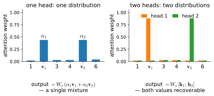
The bound is a fact about this deliberately restricted interface — one layer, with value-blind keys that mark position only — not a universal law: it lifts once a one-head model gets content-dependent keys, more depth, or a residual connection, and the copy-both separation from two heads narrows accordingly.
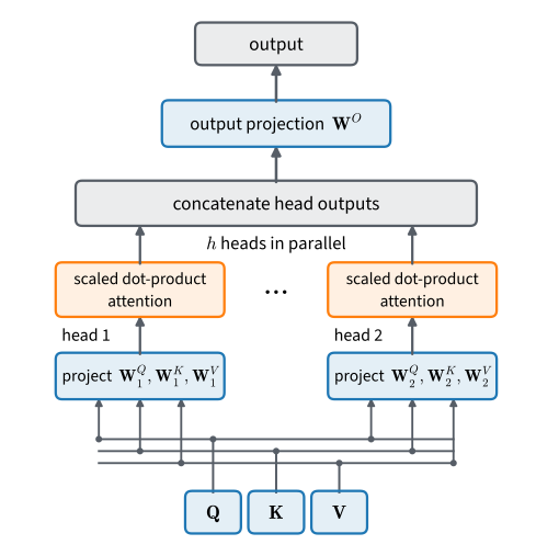
Multi-head attention addresses this limitation by assigning each query several independently parameterized attention distributions and recombining their outputs with a learned projection.
10.3.2 Multi-Head Attention
10.3.2.1 Extending to \(h\) Heads
Rather than hand-designing the heads as above, we learn them. Given a query \(\mathbf{q} \in \mathbb{R}^{d}\), keys \(\mathbf{k} \in \mathbb{R}^{d}\), and values \(\mathbf{v} \in \mathbb{R}^{d}\), head \(i\) (\(i = 1, \ldots, h\)) first projects them into its own subspace and then runs ordinary scaled dot product attention \(f\) from Section 10.2:
\[ \mathbf{h}_i = f\big(\mathbf W_i^{(q)}\mathbf q,\; \mathbf W_i^{(k)}\mathbf k,\; \mathbf W_i^{(v)}\mathbf v\big) \in \mathbb R^{p}, \tag{10.3.1}\]
with learnable \(\mathbf W_i^{(q)}, \mathbf W_i^{(k)}, \mathbf W_i^{(v)} \in \mathbb R^{p \times d}\). Because each head scores with its own projected queries and keys, each head attends according to its own notion of relevance, and each moves its own projection of the values — the two independent mixtures of the construction above, now learned and generalized to \(h\). The output is a learned linear recombination of the concatenated heads:
\[ \mathbf W_o \begin{bmatrix}\mathbf h_1\\\vdots\\\mathbf h_h\end{bmatrix} \in \mathbb{R}^{d}, \qquad \mathbf W_o \in \mathbb R^{d \times hp}. \tag{10.3.2}\]
Figure 10.3.2 shows the layout.
10.3.2.2 Parameter and FLOP Counts
The standard dimension choice makes the heads collectively no more expensive than one big head: set the per-head width to \(p = d/h\), so the \(h\) heads together produce \(hp = d\) numbers per token, exactly what a single head of width \(d\) would. For self-attention, write the sequence inputs as \(\mathbf{Q},\mathbf{K},\mathbf{V}\in\mathbb{R}^{n\times d}\); each of the four learned projections is a \(d\times d\) matrix, and each head receives matrices of shape \(n\times p\). The resulting cost is
\[ \underbrace{8nd^2}_{\textrm{projections}} \;+\; \underbrace{4n^2 d}_{\textrm{scores and mixing}} \quad \textrm{FLOPs,} \qquad 4d^2 \ \textrm{parameters,} \tag{10.3.3}\]
independent of \(h\): the four projection matrices are \(d \times d\) regardless of how their outputs are sliced into heads, and each head’s score and mixing matmuls shrink by the factor \(h\) that their count grows by (counting one multiply–add as two FLOPs). In this arithmetic, the number of heads changes the representation but not the leading operation count. Realized cost is not exactly constant because increasing the number of heads produces more, smaller matrix multiplications and softmaxes, whose kernel efficiency may differ. What does change with \(h\) is the shape of the attention map — \(h\) distributions of \(n\) weights per query instead of one.
10.3.2.3 Implementation
The per-head dimension choice also yields a standard implementation: compute one query projection of width \(d\), then reshape it into \(h\) heads of width \(d/h\), and fold the head axis into the batch axis. The attention code from Section 10.2 then runs all heads of all sequences as one big batched matrix multiplication, with no loop over heads. Within the forward pass, valid_lens is repeated \(h\) times so that each head of a sequence sees that sequence’s mask.
class MultiHeadAttention(d2l.Module):
    """Multi-head attention."""
    def __init__(self, num_hiddens, num_heads, dropout, bias=False, **kwargs):
        super().__init__()
        assert num_hiddens % num_heads == 0, 'heads must divide num_hiddens'
        self.num_heads = num_heads
        self.attention = d2l.DotProductAttention(dropout)
        self.W_q = nn.LazyLinear(num_hiddens, bias=bias)
        self.W_k = nn.LazyLinear(num_hiddens, bias=bias)
        self.W_v = nn.LazyLinear(num_hiddens, bias=bias)
        self.W_o = nn.LazyLinear(num_hiddens, bias=bias)

    def forward(self, queries, keys, values, valid_lens):
        # Shape of queries, keys, or values:
        # (batch_size, no. of queries or key-value pairs, num_hiddens)
        # Shape of valid_lens: (batch_size,) or (batch_size, no. of queries)
        queries = self.transpose_qkv(self.W_q(queries))
        keys = self.transpose_qkv(self.W_k(keys))
        values = self.transpose_qkv(self.W_v(values))

        if valid_lens is not None:
            # On axis 0, copy the first item (scalar or vector) for num_heads
            # times, then copy the next item, and so on
            valid_lens = torch.repeat_interleave(
                valid_lens, repeats=self.num_heads, dim=0)

        # Shape of output: (batch_size * num_heads, no. of queries,
        # num_hiddens / num_heads)
        output = self.attention(queries, keys, values, valid_lens)
        # Shape of output_concat: (batch_size, no. of queries, num_hiddens)
        output_concat = self.transpose_output(output)
        return self.W_o(output_concat)
class MultiHeadAttention(nnx.Module):
"""Multi-head attention."""
def __init__(self, num_hiddens, num_heads, dropout, bias=False, rngs=None):
assert num_hiddens % num_heads == 0, 'heads must divide num_hiddens'
rngs = nnx.Rngs(params=0, dropout=1) if rngs is None else rngs
self.num_hiddens, self.num_heads = num_hiddens, num_heads
self.attention = d2l.DotProductAttention(dropout, rngs=rngs)
self.W_q = nnx.Linear(num_hiddens, num_hiddens, use_bias=bias,
rngs=rngs)
self.W_k = nnx.Linear(num_hiddens, num_hiddens, use_bias=bias,
rngs=rngs)
self.W_v = nnx.Linear(num_hiddens, num_hiddens, use_bias=bias,
rngs=rngs)
self.W_o = nnx.Linear(num_hiddens, num_hiddens, use_bias=bias,
rngs=rngs)
def __call__(self, queries, keys, values, valid_lens):
# Shape of queries, keys, or values:
# (batch_size, no. of queries or key-value pairs, num_hiddens)
# Shape of valid_lens: (batch_size,) or (batch_size, no. of queries)
queries = self.transpose_qkv(self.W_q(queries))
keys = self.transpose_qkv(self.W_k(keys))
values = self.transpose_qkv(self.W_v(values))
if valid_lens is not None:
# On axis 0, copy the first item (scalar or vector) for num_heads
# times, then copy the next item, and so on
valid_lens = jnp.repeat(valid_lens, self.num_heads, axis=0)
# Shape of output: (batch_size * num_heads, no. of queries,
# num_hiddens / num_heads)
output, attention_weights = self.attention(
queries, keys, values, valid_lens)
# Shape of output_concat: (batch_size, no. of queries, num_hiddens)
output_concat = self.transpose_output(output)
# NNX idiom: return (output, weights); PyTorch returns output only
return self.W_o(output_concat), attention_weightsThe two transpositions do the head bookkeeping: transpose_qkv moves from (batch, length, num_hiddens) to (batch * num_heads, length, num_hiddens / num_heads), and transpose_output reverses it after the attention call.
@d2l.add_to_class(MultiHeadAttention)
def transpose_qkv(self, X):
    """Transposition for parallel computation of multiple attention heads."""
    # Shape of input X: (batch_size, no. of queries or key-value pairs,
    # num_hiddens). Shape of output X: (batch_size, no. of queries or
    # key-value pairs, num_heads, num_hiddens / num_heads)
    X = X.reshape(X.shape[0], X.shape[1], self.num_heads, -1)
    # Shape of output X: (batch_size, num_heads, no. of queries or key-value
    # pairs, num_hiddens / num_heads)
    X = X.permute(0, 2, 1, 3)
    # Shape of output: (batch_size * num_heads, no. of queries or key-value
    # pairs, num_hiddens / num_heads)
    return X.reshape(-1, X.shape[2], X.shape[3])

@d2l.add_to_class(MultiHeadAttention)
def transpose_output(self, X):
    """Reverse the operation of transpose_qkv."""
    X = X.reshape(-1, self.num_heads, X.shape[1], X.shape[2])
    X = X.permute(0, 2, 1, 3)
return X.reshape(X.shape[0], X.shape[1], -1)@d2l.add_to_class(MultiHeadAttention)
def transpose_qkv(self, X):
"""Transposition for parallel computation of multiple attention heads."""
# Shape of input X: (batch_size, no. of queries or key-value pairs,
# num_hiddens). Shape of output X: (batch_size, no. of queries or
# key-value pairs, num_heads, num_hiddens / num_heads)
X = X.reshape((X.shape[0], X.shape[1], self.num_heads, -1))
# Shape of output X: (batch_size, num_heads, no. of queries or key-value
# pairs, num_hiddens / num_heads)
X = jnp.transpose(X, (0, 2, 1, 3))
# Shape of output: (batch_size * num_heads, no. of queries or key-value
# pairs, num_hiddens / num_heads)
return X.reshape((-1, X.shape[2], X.shape[3]))
@d2l.add_to_class(MultiHeadAttention)
def transpose_output(self, X):
"""Reverse the operation of transpose_qkv."""
X = X.reshape((-1, self.num_heads, X.shape[1], X.shape[2]))
X = jnp.transpose(X, (0, 2, 1, 3))
return X.reshape((X.shape[0], X.shape[1], -1))A shape check: with 5 heads and 100 hidden units, batches of 2 sequences with 4 queries against 6 key–value pairs come back as (batch_size, num_queries, num_hiddens), and the per-sequence valid_lens masking flows through unchanged.
num_hiddens, num_heads = 100, 5
attention = MultiHeadAttention(num_hiddens, num_heads, 0.5)
batch_size, num_queries, num_kvpairs = 2, 4, 6
valid_lens = d2l.tensor([3, 2])
X = d2l.ones((batch_size, num_queries, num_hiddens))
Y = d2l.ones((batch_size, num_kvpairs, num_hiddens))
d2l.check_shape(attention(X, Y, Y, valid_lens),
                (batch_size, num_queries, num_hiddens))
num_hiddens, num_heads = 100, 5
attention = MultiHeadAttention(num_hiddens, num_heads, 0.5)
batch_size, num_queries, num_kvpairs = 2, 4, 6
valid_lens = d2l.tensor([3, 2])
X = d2l.ones((batch_size, num_queries, num_hiddens))
Y = d2l.ones((batch_size, num_kvpairs, num_hiddens))
d2l.check_shape(nnx.view(attention, deterministic=True)(
X, Y, Y, valid_lens)[0],
(batch_size, num_queries, num_hiddens))And the accounting of Equation 10.3.3 in the flesh: the parameter count does not move as the head count sweeps from 1 to 8.
X = d2l.ones((2, 10, 256))
for num_heads in (1, 2, 4, 8):
    attention = MultiHeadAttention(num_hiddens=256, num_heads=num_heads,
                                   dropout=0)
    attention(X, X, X, None)  # Materialize the lazily initialized layers
    print(f'{num_heads} heads: '
          f'{sum(p.numel() for p in attention.parameters())} parameters')
1 heads: 262144 parameters
2 heads: 262144 parameters
4 heads: 262144 parameters
8 heads: 262144 parametersfor num_heads in (1, 2, 4, 8):
attention = MultiHeadAttention(num_hiddens=256, num_heads=num_heads,
dropout=0)
num_params = sum(p.size for p in jax.tree.leaves(
nnx.state(attention, nnx.Param)))
print(f'{num_heads} heads: {num_params} parameters')1 heads: 262144 parameters
2 heads: 262144 parameters
4 heads: 262144 parameters
8 heads: 262144 parameters10.3.3 Self-Attention and Cross-Attention
MultiHeadAttention takes three sequence arguments: queries, keys, and values. Self-attention and cross-attention differ only in the sources of these arguments.
10.3.3.1 Self-Attention
In self-attention (Lin et al. 2017; Vaswani et al. 2017), one sequence supplies all three arguments: every token emits a query against every token’s key, and each output position is a value mixture from the same sequence. Given inputs \(\mathbf{x}_1, \ldots, \mathbf{x}_n \in \mathbb{R}^d\), the layer returns an equally long sequence \(\mathbf{y}_1, \ldots, \mathbf{y}_n\) with
\[ \mathbf{y}_i = f\big(\mathbf{x}_i,\; (\mathbf{x}_1, \mathbf{x}_1), \ldots, (\mathbf{x}_n, \mathbf{x}_n)\big) \in \mathbb{R}^d, \tag{10.3.4}\]
where \(f\) is multi-head attention pooling. Each token’s new representation combines information from the whole sequence in a single step. Transformers stack these layers because the output and input shapes agree.
num_hiddens, num_heads = 100, 5
attention = MultiHeadAttention(num_hiddens, num_heads, 0.5)
batch_size, num_queries, valid_lens = 2, 4, d2l.tensor([3, 2])
X = d2l.ones((batch_size, num_queries, num_hiddens))
d2l.check_shape(attention(X, X, X, valid_lens),
                (batch_size, num_queries, num_hiddens))
num_hiddens, num_heads = 100, 5
attention = MultiHeadAttention(num_hiddens, num_heads, 0.5)
batch_size, num_queries, valid_lens = 2, 4, d2l.tensor([3, 2])
X = d2l.ones((batch_size, num_queries, num_hiddens))
d2l.check_shape(nnx.view(attention, deterministic=True)(
X, X, X, valid_lens)[0],
(batch_size, num_queries, num_hiddens))10.3.3.2 Cross-Attention
In cross-attention, the queries come from sequence \(\mathbf{A}\), while keys and values come from sequence \(\mathbf{B}\). The output has the length of \(\mathbf{A}\) and aggregates information from \(\mathbf{B}\). This is the wiring of the original encoder–decoder transformer, where each target-language position queries the source sentence; of a vision–language model, where text tokens query image patches; and of the historical alignment models that introduced learned attention (Section 10.2). These cases use the same function with different argument sources:
A = d2l.ones((batch_size, 4, num_hiddens))
B = d2l.ones((batch_size, 9, num_hiddens))
d2l.check_shape(attention(A, B, B, None),
                (batch_size, 4, num_hiddens))
A = d2l.ones((batch_size, 4, num_hiddens))
B = d2l.ones((batch_size, 9, num_hiddens))
d2l.check_shape(nnx.view(attention, deterministic=True)(
A, B, B, None)[0],
(batch_size, 4, num_hiddens))10.3.3.3 Visualizing Cross-Attention Alignment
To visualize cross-attention, assign every letter of the alphabet a random embedding, and let the letters of one word query the letters of another through plain scaled dot product attention — no learned projections. Matching letters share an embedding, so their score concentrates near \(\sqrt{d}\) after scaling, while unrelated pairs score near zero; softmax turns this gap into a readable alignment.
words = 'attention', 'translation'
letters = sorted(set(''.join(words)))
torch.manual_seed(0)
emb = torch.randn(len(letters), 32)
queries, keys = (emb[[letters.index(c) for c in w]][None] for w in words)
attention = d2l.DotProductAttention(dropout=0)
attention(queries, keys, keys, None)
d2l.show_heatmaps(attention.attention_weights[None],
                  xlabel='keys:  t  r  a  n  s  l  a  t  i  o  n',
                  ylabel='queries:  a  t  t  e  n  t  i  o  n',
                  figsize=(4, 3.5), cmap='Blues')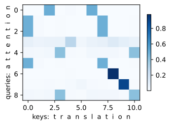
words = 'attention', 'translation'
letters = sorted(set(''.join(words)))
emb = jax.random.normal(jax.random.key(0), (len(letters), 32))
queries, keys = (emb[jnp.array([letters.index(c) for c in w])][None]
                 for w in words)
attention = d2l.DotProductAttention(dropout=0)
output, attention_weights = attention(queries, keys, keys, None)
d2l.show_heatmaps(attention_weights[None],
                  xlabel='keys:  t  r  a  n  s  l  a  t  i  o  n',
                  ylabel='queries:  a  t  t  e  n  t  i  o  n',
                  figsize=(4, 3.5), cmap='Blues')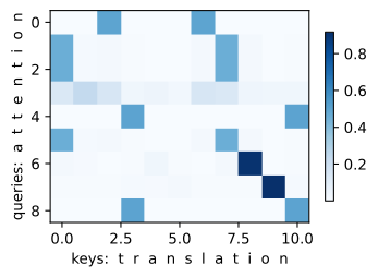
Read the map row by row (queries are the letters of “attention”, keys the letters of “translation”). Three regimes appear. The i and o queries find their unique partners and attend sharply. The a, t, and n queries find two copies each and split their weight: a single head cannot choose between identical keys, the averaging of the first section in miniature. And the e query, whose letter does not occur in “translation” at all, spreads its weight diffusely because softmax assigns all probability mass across the available keys even when none matches. Trained models show all three regimes too, which is one reason reading attention maps as explanations requires care. A diffuse row may indicate that no key is relevant rather than that all keys are relevant.
10.3.4 Summary
A single attention head gives each query one distribution over the keys and therefore one value mixture. On the value-blind copy-both task, any single head loses half the target variance. Multi-head attention computes \(h\) projected mixtures and combines them linearly. With per-head width \(d/h\), the parameter and FLOP counts are independent of \(h\); implementations can fold the head axis into the batch axis. Self-attention draws queries, keys, and values from one sequence. Cross-attention draws queries from one sequence and keys and values from another, with output length equal to the query length.
10.3.5 Exercises
- In the copy-both construction, the best linear readout loses half the variance. Does a nonlinear readout help? For Gaussian values the conditional mean is linear, so it cannot; check this numerically by training a small MLP readout on \(\mathbf{m}\) with weights \((0.5, 0.5)\). Then repeat with values drawn uniformly from \(\{-1, +1\}^d\) — explain what changes and why.
- Two heads with weights \((0.5 + \epsilon, 0.5 - \epsilon)\) and \((0.5 - \epsilon, 0.5 + \epsilon)\) still invert exactly in theory. Add Gaussian noise of standard deviation \(0.01\) to the mixtures and measure the readout error as \(\epsilon \to 0\). Relate what you see to the condition number of the \(2 \times 2\) mixing matrix.
- Feed the letter-alignment example through a freshly initialized
MultiHeadAttentionwith 4 heads instead of plain dot product attention, and plot each head’s attention map. Are the maps still readable? What does this suggest about interpreting the attention maps of a network whose projections you have not inspected? - Derive Equation 10.3.3 by counting the matrix multiplications in
MultiHeadAttention. For \(d = 512\), at which sequence length \(n\) does the quadratic score-and-mix term overtake the projection term? Later sections of this chapter take this crossover as their starting point. - Multi-query attention shares a single key and value head across all \(h\) query heads, and grouped-query attention shares them within groups. How do the parameter count and the FLOPs count of Equation 10.3.3 change under each scheme? Why is the saving most valuable during autoregressive generation?
- Suppose you want to prune the least important heads of a trained multi-head attention layer to speed up inference. Design an experiment to measure how much each head matters. How would you guard against two heads that are individually prunable but not jointly?