%matplotlib inline
from d2l import torch as d2l
import numpy as np29.3 The Fokker–Planck Equation and Probability Flow
A path generated by a stochastic differential equation is random and nowhere differentiable. Its marginal density \(p_t(\mathbf{x})\), however, evolves deterministically. Drift transports this density and diffusion smooths it. The partial differential equation governing this evolution is the Fokker–Planck equation. This shift from individual paths to the ensemble density is central to diffusion models.
The Fokker–Planck equation yields two constructions. The probability-flow ODE has smooth deterministic trajectories and the same time-marginals \(p_t\) as the original SDE (Song et al. 2021). The reverse of the noising process is another SDE whose drift depends on the score \(\nabla_{\mathbf{x}} \log p_t(\mathbf{x})\) (Anderson 1982). The forward drift \(\mathbf{f}\) and noise schedule \(g\) are known by design, so the score is the quantity that must be estimated from data in Section 29.4.
We first distinguish pathwise and density evolution and review the required vector-calculus identities: divergence, the Laplacian, and integration by parts in \(d\) dimensions. We then derive the Fokker–Planck equation from Itô’s lemma, check it in closed form and numerically on the Ornstein–Uhlenbeck process, rewrite it as a continuity equation and identify the probability-flow ODE. We then derive scores for Gaussians and mixtures, establish their invariance to the normalizing constant, and apply Anderson’s time-reversal theorem. The numerical examples use NumPy and closed-form densities; no model is trained in this section.
%matplotlib inline
from d2l import tensorflow as d2l
import numpy as np%matplotlib inline
from d2l import jax as d2l
import numpy as np%matplotlib inline
from d2l import mxnet as d2l
import numpy as np29.3.1 From Paths to Densities
29.3.1.1 Pathwise and Ensemble Views
Fix an SDE in the form we will use throughout,
\[ d\mathbf{X} = \mathbf{f}(\mathbf{X}, t)\,dt + g(t)\,d\mathbf{W}, \]
with drift \(\mathbf{f} : \mathbb{R}^d \times [0, T] \to \mathbb{R}^d\) and a scalar noise schedule \(g(t)\), and start it from a random initial condition \(\mathbf{X}_0 \sim p_0\). There are two ways to analyze its evolution.
The Lagrangian view follows one particle: a single realization of the Brownian motion produces a single path \(\mathbf{X}_t(\omega)\), different on every run. The Eulerian view instead fixes a point \(\mathbf{x}\) and tracks the time-marginal \(p_t(\mathbf{x})\), the density of the random variable \(\mathbf{X}_t\). The marginal averages over both sources of randomness (the draw of \(\mathbf{X}_0\) and the noise along the way), and that averaging is exactly what makes it deterministic. Repeated large-cloud experiments estimate the same evolving density, even though their individual paths differ.
Our running example is the Ornstein–Uhlenbeck (OU) process of Section 29.2.4, \(dX = -\theta X\,dt + \sigma\,dW\), whose marginals we know in closed form: started from a point \(X_0 = x_0\),
\[ X_t \sim \mathcal{N}\!\left(x_0 e^{-\theta t},\; \frac{\sigma^2}{2\theta}\left(1 - e^{-2\theta t}\right)\right), \tag{29.3.1}\]
the transition kernel Equation 29.2.14, restated here for repeated use: a Gaussian whose mean decays toward the origin and whose variance saturates at the stationary value \(\sigma^2 / 2\theta\) derived in Section 29.2.4. Qualitatively, the drift transports probability mass (the cloud’s center of mass slides along the deterministic flow \(\dot{x} = -\theta x\)), while the diffusion spreads and smooths it (the cloud widens the way heat spreads along a metal bar). The Fokker–Planck equation will make both halves of that sentence into operators.
29.3.1.2 Three Identities from Vector Calculus
Beyond the gradient of Section 25.2, the derivation uses three vector-calculus identities about a smooth vector field \(\mathbf{v} : \mathbb{R}^d \to \mathbb{R}^d\) and a smooth scalar field \(h : \mathbb{R}^d \to \mathbb{R}\). Together they provide the required analytic tools.
Divergence. The divergence of \(\mathbf{v}\) is the scalar field
\[ \nabla \cdot \mathbf{v} = \sum_{i=1}^d \frac{\partial v_i}{\partial x_i}. \tag{29.3.2}\]
Its meaning is flux per unit volume: if \(\mathbf{v}\) is the velocity of a fluid, then \(\nabla \cdot \mathbf{v}(\mathbf{x})\) is the net rate at which fluid exits an infinitesimal box around \(\mathbf{x}\), divided by the box’s volume: positive at a source, negative at a sink, zero for an incompressible flow. The local statement integrates up to the divergence theorem: for a bounded region \(\Omega\) with outward unit normal \(\mathbf{n}\),
\[ \int_\Omega \nabla \cdot \mathbf{v}\; d\mathbf{x} = \oint_{\partial\Omega} \mathbf{v} \cdot \mathbf{n}\; dS, \tag{29.3.3}\]
Thus, the integrated divergence over a region equals the net outward boundary flux. In one dimension this is just the fundamental theorem of calculus, \(\int_a^b v'(x)\,dx = v(b) - v(a)\): what accumulates inside \([a, b]\) is whatever crosses the two endpoints. We take the divergence theorem itself as a granted fact; a proof is in Folland (1999) .
Laplacian. The Laplacian is the divergence of the gradient,
\[ \Delta h = \nabla \cdot (\nabla h) = \sum_{i=1}^d \frac{\partial^2 h}{\partial x_i^2}. \tag{29.3.4}\]
It measures how \(h\) at a point compares with its neighborhood: averaging \(h\) over a small sphere of radius \(r\) centered at \(\mathbf{x}\) gives \(h(\mathbf{x}) + \frac{r^2}{2d}\Delta h(\mathbf{x}) + O(r^4)\). So \(\Delta h > 0\) means “below the neighborhood average.” That is why the heat equation \(\partial_t u = \Delta u\) smooths: it raises \(u\) exactly where \(u\) sits below the average of its neighbors, and lowers it where it sits above.
Integration by parts. This is the \(d\)-dimensional form of the one-dimensional rule of Section 25.4.2.2. If \(h\) and \(\mathbf{v}\) are smooth and decay fast enough at infinity (for us: \(h\) a compactly supported test function, or Gaussian-tailed densities), then
\[ \int h\, (\nabla \cdot \mathbf{v})\; d\mathbf{x} = -\int \nabla h \cdot \mathbf{v}\; d\mathbf{x}. \tag{29.3.5}\]
Proof in one line: the product rule gives \(\nabla \cdot (h \mathbf{v}) = \nabla h \cdot \mathbf{v} + h\, \nabla \cdot \mathbf{v}\); integrate both sides over a ball of radius \(R\) and let \(R \to \infty\): by the divergence theorem the left side is a boundary flux of \(h\mathbf{v}\), which vanishes under the decay assumption. \(\blacksquare\)
Applied twice with \(\mathbf{v} = \nabla u\), integration by parts moves a whole Laplacian across the integral sign: \(\int h\, \Delta u = \int u\, \Delta h\). This identity shifts derivatives from a test function onto a density, which is the main step in the Fokker–Planck derivation.
29.3.1.3 Simulating the Marginal Density
Before the derivation, a simulation illustrates that the marginal is deterministic and, for OU, exactly the Gaussian 2. We initialize \(100{,}000\) particles at \(x_0 = 2\), simulate them with Euler–Maruyama (Section 29.2.3.2), and compare histograms of the cloud against the analytic density at three times. We take \(\theta = 1\) and \(\sigma = \sqrt{2}\) throughout, so the stationary law is exactly \(\mathcal{N}(0, 1)\).
theta, sigma = 1.0, np.sqrt(2.0)        # OU: dX = -theta X dt + sigma dW

def ou_mean_var(x0, t):                 # closed-form marginal N(m_t, v_t)
    m = x0 * np.exp(-theta * t)
    v = sigma**2 / (2 * theta) * (1 - np.exp(-2 * theta * t))
    return m, v

rng = np.random.default_rng(42)
n, dt, T = 100_000, 0.002, 2.0
cloud = np.full(n, 2.0)                 # every particle starts at x0 = 2
ts_show, snaps = (0.1, 0.5, 2.0), {}
for k in range(int(round(T / dt))):
    cloud += -theta * cloud * dt + sigma * np.sqrt(dt) * rng.standard_normal(n)
    t = (k + 1) * dt
    if any(abs(t - s) < 1e-9 for s in ts_show):
        snaps[round(t, 3)] = cloud.copy()

grid = np.linspace(-3.5, 4.5, 400)
d2l.set_figsize((6, 2.5))
for t, color in zip(ts_show, ('C0', 'C1', 'C2')):
    m, v = ou_mean_var(2.0, t)
    d2l.plt.hist(snaps[t], bins=80, density=True, alpha=0.35, color=color)
    d2l.plt.plot(grid, np.exp(-(grid - m)**2 / (2 * v)) / np.sqrt(2 * np.pi * v),
                 color=color, label=f't = {t}')
    print(f't={t}: cloud mean {snaps[t].mean():+.4f} (analytic {m:+.4f}), '
          f'std {snaps[t].std():.4f} (analytic {np.sqrt(v):.4f})')
d2l.plt.xlabel('x'); d2l.plt.ylabel('density'); d2l.plt.legend();t=0.1: cloud mean +1.8121 (analytic +1.8097), std 0.4275 (analytic 0.4258)
t=0.5: cloud mean +1.2137 (analytic +1.2131), std 0.7987 (analytic 0.7951)
t=2.0: cloud mean +0.2750 (analytic +0.2707), std 0.9889 (analytic 0.9908)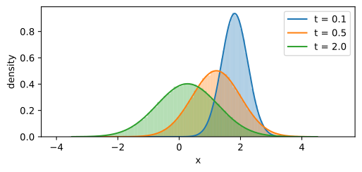
t=0.1: cloud mean +1.8121 (analytic +1.8097), std 0.4275 (analytic 0.4258)
t=0.5: cloud mean +1.2137 (analytic +1.2131), std 0.7987 (analytic 0.7951)
t=2.0: cloud mean +0.2750 (analytic +0.2707), std 0.9889 (analytic 0.9908)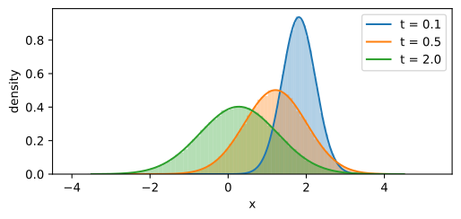
t=0.1: cloud mean +1.8121 (analytic +1.8097), std 0.4275 (analytic 0.4258)
t=0.5: cloud mean +1.2137 (analytic +1.2131), std 0.7987 (analytic 0.7951)
t=2.0: cloud mean +0.2750 (analytic +0.2707), std 0.9889 (analytic 0.9908)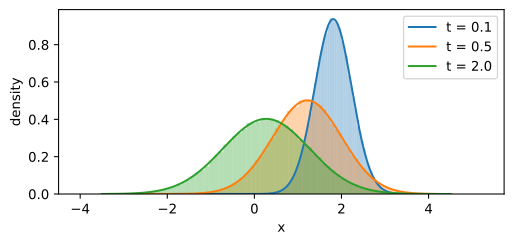
t=0.1: cloud mean +1.8121 (analytic +1.8097), std 0.4275 (analytic 0.4258)
t=0.5: cloud mean +1.2137 (analytic +1.2131), std 0.7987 (analytic 0.7951)
t=2.0: cloud mean +0.2750 (analytic +0.2707), std 0.9889 (analytic 0.9908)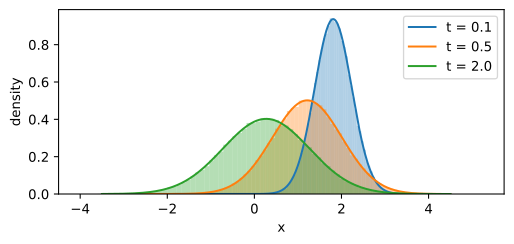
The histograms match their analytic densities: at \(t = 0.5\) the cloud’s mean \(1.2137\) and standard deviation \(0.7987\) match the analytic \(2e^{-0.5} \approx 1.2131\) and \(\sqrt{1 - e^{-1}} \approx 0.7951\) to within a few parts in a thousand (the gap is Euler–Maruyama discretization plus sampling noise), and by \(t = 2\) the cloud is already close to the stationary \(\mathcal{N}(0, 1)\). Despite random individual paths, the ensemble estimates one deterministic time-dependent density. The next subsection derives its PDE.
29.3.2 The Fokker–Planck Equation
29.3.2.1 From Itô’s Lemma to a PDE
Although an SDE path is not differentiable, the expectation of a smooth test function along the path can be differentiated using Itô’s lemma (Section 29.2.2.3). Equality against every smooth test function then determines the density evolution.
Take any smooth, compactly supported test function \(\phi : \mathbb{R}^d \to \mathbb{R}\). For \(d\mathbf{X} = \mathbf{f}\,dt + g\,d\mathbf{W}\), the multivariate Itô lemma Equation 29.2.8 with \(G = g(t)\, I\) reads
\[ d\phi(\mathbf{X}) = \left(\nabla\phi \cdot \mathbf{f} + \tfrac12 g^2 \Delta\phi\right) dt + g\, \nabla\phi \cdot d\mathbf{W} : \]
the ordinary chain rule plus the second-order Taylor term that \((dW)^2 = dt\) promotes to first order; with scalar \(g\), that correction \(\tfrac12 \sum_{ij} (G G^\top)_{ij}\, \partial^2_{x_i x_j}\phi\) collapses to exactly \(\tfrac12 g^2\) times the Laplacian of \(\phi\). Now take expectations. The Itô integral has zero mean (Section 29.2.2.3), so the noise term vanishes and
\[ \frac{d}{dt}\, \mathbb{E}[\phi(\mathbf{X}_t)] = \mathbb{E}\!\left[\nabla\phi \cdot \mathbf{f} + \tfrac12 g^2 \Delta\phi\right]. \]
Both sides are integrals against the marginal density: writing \(\mathbb{E}[\,\cdot\,] = \int (\cdot)\, p_t(\mathbf{x})\, d\mathbf{x}\),
\[ \int \phi\; \partial_t p_t\; d\mathbf{x} = \int (\nabla\phi \cdot \mathbf{f})\, p_t\; d\mathbf{x} + \tfrac12 g^2 \int (\Delta\phi)\, p_t\; d\mathbf{x}. \]
Integration by parts Equation 29.3.5 transfers the derivatives from \(\phi\) to \(p_t\). Applied once to the drift term (with \(h = \phi\), \(\mathbf{v} = \mathbf{f} p_t\)) and twice to the diffusion term,
\[ \int \phi\, \partial_t p_t\; d\mathbf{x} = \int \phi \left[-\nabla \cdot (\mathbf{f}\, p_t) + \tfrac12 g^2 \Delta p_t\right] d\mathbf{x}. \]
This holds for every test function \(\phi\). Here we fix the standing assumptions of the whole section: \(p_t\) is smooth and strictly positive, differentiation under the integral sign is justified, and \(p_t\) decays fast enough at infinity that the products \(\mathbf{f}\, p_t\) and \(\nabla p_t\) vanish there. (The decay must cover the products: the OU drift grows linearly, so it is \(\mathbf{f}\, p_t\), not \(p_t\) alone, that has to vanish; Gaussian tails oblige.) Under these assumptions both integrands are continuous, and a continuous function that integrates to zero against every test function is identically zero, so the integrands agree pointwise and \(p_t\) solves the resulting PDE classically. That PDE is the Fokker–Planck equation (Fokker 1914; Planck 1917) (also the Kolmogorov forward equation (Kolmogorov 1931); physicists’ conventions and many generalizations are in Risken (1996)):
\[ \partial_t p_t(\mathbf{x}) = -\nabla \cdot \big(\mathbf{f}(\mathbf{x}, t)\, p_t(\mathbf{x})\big) + \tfrac12 g(t)^2\, \Delta p_t(\mathbf{x}). \tag{29.3.6}\]
For a full matrix diffusion \(G(\mathbf{x}, t)\,d\mathbf{W}\), put \(a=GG^\top\). The second-order term is then \(\tfrac12 \sum_{ij} \partial_i\partial_j(a_{ij}p_t)\). The scalar-\(g\) case used in most examples is the special choice \(a=g(t)^2I\), for which this reduces to \(\tfrac12 g(t)^2\Delta p_t\).
29.3.2.2 Diffusion Matrices and Boundary Conditions
The matrix formula becomes easier to interpret when written as conservation of probability. Define the probability current componentwise by
\[ J_i(\mathbf{x},t) = f_i(\mathbf{x},t)p_t(\mathbf{x}) - \frac12\sum_j \partial_j\big(a_{ij}(\mathbf{x},t)p_t(\mathbf{x})\big). \]
Then the general Fokker–Planck equation is \(\partial_t p_t=-\nabla\cdot\mathbf{J}\). Integrating it over a domain \(\Omega\) gives
\[ \frac{d}{dt}\int_\Omega p_t(\mathbf{x})\,d\mathbf{x} = -\int_{\partial\Omega}\mathbf{J}\cdot\mathbf{n}\,dS. \]
This identity makes the required boundary assumptions explicit. On all of \(\mathbb{R}^d\) we require the current to decay sufficiently fast. A reflecting boundary imposes \(\mathbf{J}\cdot\mathbf{n}=0\); periodic boundaries match density and flux on opposite faces. A common absorbing condition is \(p=0\) on the boundary, in which case probability may leave the domain and the integral of \(p\) need not remain one unless an absorbed state is included. Integration by parts without the matching boundary term is not valid in these settings.
Where \(p_t>0\), dividing the current by the density gives the general probability-flow velocity
\[ \mathbf{v} = \frac{\mathbf{J}}{p_t} = \mathbf{f}-\frac12\,a\nabla\log p_t -\frac12\,\nabla\cdot a, \qquad (\nabla\cdot a)_i=\sum_j\partial_j a_{ij}. \]
Thus state-dependent or anisotropic noise contributes both a score term and a spatial-divergence term. The later formula \(\mathbf{f}-\tfrac12g^2\nabla\log p_t\) is precisely the simplification for \(a=g(t)^2I\).
| Diffusion | Fokker–Planck second-order term | Probability-flow correction to \(\mathbf f\) |
|---|---|---|
| \(g(t)I\) | \(\tfrac12g(t)^2\Delta p\) | \(-\tfrac12g(t)^2\nabla\log p\) |
| \(G(\mathbf x,t)\), \(a=GG^\top\) | \(\tfrac12\sum_{ij}\partial_i\partial_j(a_{ij}p)\) | \(-\tfrac12a\nabla\log p-\tfrac12\nabla\cdot a\) |
The second row requires the derivatives and boundary conditions used in the probability-current derivation; it cannot be obtained by replacing scalar \(g^2\) with a matrix while leaving the rest of the formula unchanged.
29.3.2.3 Drift and Diffusion Terms
Equation Equation 29.3.6 contains two distinct terms. The first term, \(-\nabla \cdot (\mathbf{f} p)\), is advection: probability is transported along the drift field. The next section identifies this term with pure transport. The second term, \(\tfrac12 g^2 \Delta p\), is diffusion: by the neighborhood-average reading of the Laplacian, it increases density below the local average and decreases density above the local average. It is the \((dW)^2 = dt\) correction of Itô’s lemma made macroscopic.
Switch the drift off entirely and the Fokker–Planck equation is the heat equation,
\[ \mathbf{f} = \mathbf{0} : \qquad \partial_t p_t = \tfrac12 g^2\, \Delta p_t, \tag{29.3.7}\]
whose Gaussian solutions spread with linearly growing variance \(v(t) = v_0 + g^2 t\), precisely the \(\mathrm{Var}(W_t) = t\) law of Brownian motion from Section 29.2 (with \(g \equiv 1\)). Diffusion models’ “variance-exploding” forward process (Section 29.2) is exactly this equation with a time-dependent \(g\).
29.3.2.4 The Ornstein–Uhlenbeck Check
For OU in one dimension, with \(f(x) = -\theta x\) and \(g = \sigma\), equation Equation 29.3.6 reads
\[ \partial_t p = \theta\, \partial_x (x\, p) + \tfrac12 \sigma^2\, \partial_{xx} p, \]
The Gaussian marginal 2 solves this equation. Substituting a generic Gaussian identifies the complete Gaussian solution family and reduces the PDE to two ODEs for the mean and variance.
Proposition (Gaussian solutions of the OU equation). Let \(p(x, t) = \mathcal{N}(x; m(t), v(t))\) be a Gaussian density with differentiable mean \(m(t)\) and variance \(v(t) > 0\). Then \(p\) solves the OU Fokker–Planck equation if and only if
\[ \dot{m} = -\theta m, \qquad \dot{v} = \sigma^2 - 2\theta v. \tag{29.3.8}\]
Proof. For a Gaussian, \(\partial_x p = -\frac{x - m}{v}\, p\). Direct differentiation turns each side of the PDE into \(p\) times a quadratic polynomial in \((x - m)\):
\[ \partial_t p = p \left[\frac{\dot m}{v}(x - m) + \frac{\dot v}{2v^2}\big((x - m)^2 - v\big)\right], \]
while, writing \(x = (x - m) + m\) in the drift term,
\[ \theta\, \partial_x(x p) + \tfrac{\sigma^2}{2} \partial_{xx} p = p \left[-\frac{\theta m}{v}(x - m) + \Big(\frac{\sigma^2}{2v^2} - \frac{\theta}{v}\Big)\big((x - m)^2 - v\big)\right]. \]
The functions \(1, (x - m), (x - m)^2\) are linearly independent, so the two sides agree for all \(x\) exactly when the coefficients match: \(\dot{m} = -\theta m\) from the linear term and \(\dot{v} = \sigma^2 - 2\theta v\) from the quadratic term (the constant term repeats the latter). \(\blacksquare\)
The OU marginal 2 has \(m(t) = x_0 e^{-\theta t}\) and \(v(t) = \frac{\sigma^2}{2\theta}(1 - e^{-2\theta t})\), which satisfy Equation 29.3.8 on sight, so the transition density of Section 29.2.4 solves Fokker–Planck, by direct differentiation. The fixed point \(\dot m = \dot v = 0\) gives \(m = 0\), \(v = \sigma^2/2\theta\): the stationary Gaussian is the steady state \(\partial_t p = 0\) of the PDE (you will re-derive it from scratch, without the Gaussian ansatz, in the exercises). And setting \(\theta = 0\) recovers the heat equation’s linear variance growth \(\dot v = \sigma^2\).
A finite-difference calculation independently checks the closed-form result. We evaluate both sides of the PDE by finite differences on a grid (\(\partial_t\) by a centered difference in time, \(\partial_x\) and \(\partial_{xx}\) by np.gradient) and measure the residual.
def ou_density(x, t, x0=2.0):
    m, v = ou_mean_var(x0, t)
    return np.exp(-(x - m)**2 / (2 * v)) / np.sqrt(2 * np.pi * v)

xs = np.linspace(-4.0, 5.0, 4001)
dx = xs[1] - xs[0]
for t in ts_show:
    eps = 1e-5
    dpdt = (ou_density(xs, t + eps) - ou_density(xs, t - eps)) / (2 * eps)
    p = ou_density(xs, t)
    transport = np.gradient(theta * xs * p, dx)        # -d/dx(f p), f = -theta x
    diffusion = 0.5 * sigma**2 * np.gradient(np.gradient(p, dx), dx)
    residual = (dpdt - (transport + diffusion))[5:-5]  # trim one-sided edge stencils
    print(f't={t}: max|residual| = {np.abs(residual).max():.2e}, '
          f'max|dp/dt| = {np.abs(dpdt).max():.2e}')
t=0.1: max|residual| = 1.34e-04, max|dp/dt| = 4.82e+00
t=0.5: max|residual| = 4.56e-06, max|dp/dt| = 5.40e-01
t=2.0: max|residual| = 1.08e-06, max|dp/dt| = 6.70e-02At every time the residual is four to five orders of magnitude below the scale of \(\partial_t p\) (at \(t = 0.5\), a residual of \(5 \times 10^{-6}\) against a left-hand side of size \(0.54\)): pure finite-difference truncation error. Thus the evolving empirical density is consistent with Equation 29.3.6 at the tested resolution.
One further reading, for later context: for a gradient drift \(\mathbf{f} = -\nabla V\) and constant \(g\), the Fokker–Planck equation is the steepest-descent flow of a free-energy functional in the Wasserstein geometry of optimal transport (Section 28.2.3.3), a result of Jordan et al. (1998) . We will not use this, but it is why transport mathematics keeps resurfacing here, from the continuity equation below to the Benamou–Brenier principle (Benamou and Brenier 2000) that Section 29.4 builds on.
29.3.3 The Continuity Equation and the Probability-Flow ODE
29.3.3.1 Conservation of Probability
Forget noise for a moment. Suppose particles move deterministically, each one following a velocity field: \(\dot{\mathbf{x}} = \mathbf{v}(\mathbf{x}, t)\). What PDE does their density \(q_t\) obey? Probability mass is never created or destroyed: the amount inside any fixed region \(\Omega\) can change only by mass flowing across the boundary. Particles cross a boundary patch at rate (density) \(\times\) (velocity), so the flux density is \(q\mathbf{v}\), and
\[ \frac{d}{dt} \int_\Omega q_t\; d\mathbf{x} = -\oint_{\partial\Omega} q_t\, \mathbf{v} \cdot \mathbf{n}\; dS = -\int_\Omega \nabla \cdot (q_t \mathbf{v})\; d\mathbf{x}, \]
the divergence theorem Equation 29.3.3 converting the boundary flux into a volume integral. Since \(\Omega\) is arbitrary, the integrands agree pointwise. The result is the continuity equation:
\[ \partial_t q_t + \nabla \cdot (q_t\, \mathbf{v}) = 0. \tag{29.3.9}\]
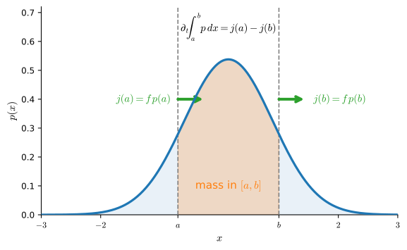
It is the same conservation law that governs fluids and electric charge. The flux density \(\mathbf{j} = q\, \mathbf{v}\) is called the probability current: at each point it gives the rate, per unit area, at which probability crosses a surface placed there. In one dimension the current makes the bookkeeping vivid, \(\partial_t \int_a^b q\,dx = j(a) - j(b)\): what flows in at \(a\) minus what leaks out at \(b\). Figure 29.3.1 draws exactly this balance.
Two consequences follow. Integrating Equation 29.3.9 over all of \(\mathbb{R}^d\) makes the divergence term vanish because the flux of \(q_t \mathbf{v}\) at infinity is zero under the decay assumption. Thus total mass \(\int q_t = 1\) is conserved. Along a flow trajectory, a particle’s log-density changes at minus the local divergence,
\[ \frac{d}{dt} \log q_t(\mathbf{x}(t)) = -\nabla \cdot \mathbf{v}(\mathbf{x}(t), t) : \]
this is the instantaneous change-of-variables formula Equation 29.1.9, proved in 1; in the present language it is just the continuity equation with its divergence expanded and read along characteristics. We are about to make diffusion models eligible for it.
29.3.3.2 Rewriting Diffusion as Transport
The Fokker–Planck equation Equation 29.3.6 is not initially in continuity form: alongside the transport term \(-\nabla \cdot (\mathbf{f} p)\) it contains a Laplacian. Wherever \(p > 0\), the chain rule gives
\[ \nabla p = p\, \nabla \log p, \tag{29.3.10}\]
and therefore
\[ \tfrac12 g^2\, \Delta p = \tfrac12 g^2\, \nabla \cdot (\nabla p) = \nabla \cdot \big(p \cdot \tfrac12 g^2 \nabla \log p\big). \tag{29.3.11}\]
The standalone rewrite Equation 29.3.11 carries a plus: the diffusion term equals the divergence of \(p\) times \(+\tfrac12 g^2 \nabla \log p\). The familiar minus sign appears only at the next step, when we fold this term into the continuity form \(-\nabla \cdot (p\, \mathbf{v})\) and the velocity absorbs it as \(-\tfrac12 g^2 \nabla \log p\). (Putting the minus in both places is a popular way to derive a contradiction.)
Proposition (Fokker–Planck is a continuity equation). Wherever \(p_t > 0\), the Fokker–Planck equation Equation 29.3.6 is equivalent to
\[ \partial_t p_t + \nabla \cdot (p_t\, \mathbf{v}_t) = 0, \qquad \mathbf{v}_t(\mathbf{x}) = \mathbf{f}(\mathbf{x}, t) - \tfrac12 g(t)^2\, \nabla \log p_t(\mathbf{x}). \tag{29.3.12}\]
Proof. Substitute Equation 29.3.11 into Equation 29.3.6 and merge the two divergences:
\[ \partial_t p = -\nabla \cdot (\mathbf{f} p) + \nabla \cdot \big(p \cdot \tfrac12 g^2 \nabla \log p\big) = -\nabla \cdot \big(p\, [\mathbf{f} - \tfrac12 g^2 \nabla \log p]\big). \qquad \blacksquare \]
At the level of densities, the diffusion therefore has the same evolution as particles moving deterministically with effective velocity \(\mathbf{v}_t\). The score correction points down the density gradient and reproduces the smoothing effect of diffusion. We check the identity numerically by comparing both sides of Equation 29.3.11 on a grid, for the OU Gaussian, along with the sign-flipped impostor.
p = ou_density(xs, 0.5)
lhs = 0.5 * sigma**2 * np.gradient(np.gradient(p, dx), dx)
score_fd = np.gradient(np.log(p), dx)
rhs = np.gradient(p * (0.5 * sigma**2 * score_fd), dx)      # correct: + sign
wrong = np.gradient(p * (-0.5 * sigma**2 * score_fd), dx)   # sign-flipped
trim = slice(5, -5)                                         # drop edge stencils
print(f'max|lhs| = {np.abs(lhs[trim]).max():.3e}')
print(f'max|lhs - rhs|   (plus sign)  = {np.abs((lhs - rhs)[trim]).max():.3e}')
print(f'max|lhs - wrong| (minus sign) = {np.abs((lhs - wrong)[trim]).max():.3e}')
max|lhs| = 7.938e-01
max|lhs - rhs| (plus sign) = 3.179e-06
max|lhs - wrong| (minus sign) = 1.588e+00The correct identity holds to finite-difference precision (the two sides agree to \(3 \times 10^{-6}\) on terms of size \(0.79\), five orders of magnitude), while the sign-flipped version misses by \(1.59\), twice the size of the term itself, exactly as \(-x\) misses \(x\). Signs matter.
29.3.3.3 The Probability-Flow ODE
A continuity equation is the law of motion of a deterministic flow. Rewriting the Fokker–Planck equation in this form identifies an ODE whose particles sweep out the same evolving density as the SDE’s random walkers:
\[ \frac{d\mathbf{x}}{dt} = \mathbf{v}_t(\mathbf{x}) = \mathbf{f}(\mathbf{x}, t) - \tfrac12 g(t)^2\, \nabla \log p_t(\mathbf{x}), \tag{29.3.13}\]
the probability-flow ODE of Song et al. (2021).
Proposition (the deterministic twin). Let \(p_t\) be the (smooth, positive, decaying) solution of the Fokker–Planck equation for the SDE \(d\mathbf{X} = \mathbf{f}\,dt + g\,d\mathbf{W}\) with \(\mathbf{X}_0 \sim p_0\). Let \(\mathbf{x}(t)\) solve the ODE Equation 29.3.13 with \(\mathbf{x}(0) \sim p_0\). Then \(\mathbf{x}(t) \sim p_t\) for every \(t\): the ODE and the SDE share all time-marginals.
Proof. Let \(q_t\) be the density of the ODE’s state. The field \(\mathbf{v}_t\) is a fixed, known velocity field (built from \(p\), not from \(q\)), so \(q_t\) obeys the continuity equation \(\partial_t q = -\nabla \cdot (q \mathbf{v}_t)\), a linear transport PDE in \(q\). By the previous proposition, \(p_t\) solves the same PDE, and both start from the same initial density \(q_0 = p_0\). A linear transport equation with a smooth velocity field determines its solution uniquely: run the characteristics \(\dot{\mathbf{x}} = \mathbf{v}_t(\mathbf{x})\), which for a locally Lipschitz velocity field cover space bijectively (Section 29.1.1.3), and the density everywhere is pinned down by change of variables along them. Here we take as granted that the characteristics exist for all time, i.e. do not blow up in finite time; that holds for the fields of this section, whose growth at infinity is at most linear (the OU drift, and the score of a Gaussian or of a Gaussian mixture). Hence \(q_t = p_t\). \(\blacksquare\)
First, marginals agree; paths do not. An SDE path is jagged, crosses itself, and re-randomizes at every instant; an ODE trajectory is smooth and, by uniqueness (Section 29.1), can never cross another one. The two processes transport the same crowd in entirely different ways.
Second, the ODE is invertible under the hypotheses above and has an exact along-trajectory likelihood identity. Integrating it from \(0\) to \(T\) gives
\[ \log p_0(\mathbf{x}(0)) = \log p_T(\mathbf{x}(T)) + \int_0^T \nabla \cdot \mathbf{v}_t(\mathbf{x}(t))\; dt, \tag{29.3.14}\]
which is the instantaneous change of variables of 1 applied to the probability-flow field. With the exact score, a known exact terminal density, exact divergence, and exact ODE integration, it evaluates the model likelihood exactly. A learned score, Hutchinson trace estimate, or numerical solver introduces approximation; this is the route used to estimate diffusion-model likelihoods (Song et al. 2021).
Third, look at Equation 29.3.13. We chose \(\mathbf{f}\), we chose \(g\). The only quantity in the probability-flow velocity that we do not know is \(\nabla \log p_t\).
29.3.3.4 Comparing SDE and ODE Marginals
We take a bimodal initial density (a two-component Gaussian mixture, the cartoon of “data”) and push it through the OU process. OU maps Gaussian mixtures to Gaussian mixtures in closed form: each component’s mean and variance follows 2, so \(p_t\), and hence its score, is available analytically at every time. (We implement the score with the numerically stable softmax trick; the formula itself is derived below, in the score-function section.)
pis = np.array([0.5, 0.5])              # data density p0: bimodal mixture
mus = np.array([-2.0, 2.0])
s2s = np.array([0.25**2, 0.25**2])

def mixture_params(t):                  # OU evolves each component in closed form
    m = mus * np.exp(-theta * t)
    v = s2s * np.exp(-2 * theta * t) + sigma**2 / (2 * theta) * (
        1 - np.exp(-2 * theta * t))
    return m, v

def gauss(x, m, v):
    return np.exp(-(x - m)**2 / (2 * v)) / np.sqrt(2 * np.pi * v)

def p_t(x, t):                          # the exact marginal density at time t
    m, v = mixture_params(t)
    return sum(pi * gauss(x, mi, vi) for pi, mi, vi in zip(pis, m, v))

def score_t(x, t):                      # exact score via stable responsibilities
    m, v = mixture_params(t)
    logw = np.stack([np.log(pi) - 0.5 * np.log(2 * np.pi * vi)
                     - (x - mi)**2 / (2 * vi)
                     for pi, mi, vi in zip(pis, m, v)])
    logw -= logw.max(axis=0)            # stable softmax over components
    w = np.exp(logw); w /= w.sum(axis=0)
    comp_scores = np.stack([-(x - mi) / vi for mi, vi in zip(m, v)])
    return (w * comp_scores).sum(axis=0)

def sample_p0(n, rng):
    k = rng.random(n) < pis[0]
    comp = np.where(k, 0, 1)
    return mus[comp] + np.sqrt(s2s[comp]) * rng.standard_normal(n)

wide, dxw = np.linspace(-8, 8, 4001), 16 / 4000
for t in (0.0, 1.0, 3.0):               # continuity: total mass is conserved
    print(f'integral of p_t at t={t}: {p_t(wide, t).sum() * dxw:.6f}')
integral of p_t at t=0.0: 1.000000
integral of p_t at t=1.0: 1.000000
integral of p_t at t=3.0: 1.000000Mass check passed: \(\int p_t = 1\) at every time, as the continuity equation promised. Now the experiment: from one shared sample of \(p_0\) we launch two clouds. The first follows the SDE with Euler–Maruyama steps; the second follows the probability-flow ODE Equation 29.3.13 with Heun steps (Section 29.1), using the exact score. We overlay marginal histograms at three times and measure the largest gap between the two clouds’ empirical CDFs (the Kolmogorov–Smirnov distance).
def pf_velocity(x, t):                  # v = f - (1/2) g^2 score
    return -theta * x - 0.5 * sigma**2 * score_t(x, t)

def ks_distance(a, b):                  # max gap between empirical CDFs
    zs = np.sort(np.concatenate([a, b]))
    Fa = np.searchsorted(np.sort(a), zs, side='right') / len(a)
    Fb = np.searchsorted(np.sort(b), zs, side='right') / len(b)
    return np.abs(Fa - Fb).max()

rng = np.random.default_rng(0)
n, T, steps = 20_000, 3.0, 600
dt = T / steps
x_sde = sample_p0(n, rng); x_ode = x_sde.copy()
ts_show, snaps_sde, snaps_ode = (0.25, 1.0, 3.0), {}, {}
paths_sde, paths_ode = [x_sde[:8].copy()], [x_ode[:8].copy()]
for k in range(steps):
    t = k * dt
    x_sde += -theta * x_sde * dt + sigma * np.sqrt(dt) * rng.standard_normal(n)
    k1 = pf_velocity(x_ode, t)          # Heun (improved Euler) for the ODE
    k2 = pf_velocity(x_ode + dt * k1, t + dt)
    x_ode += 0.5 * dt * (k1 + k2)
    paths_sde.append(x_sde[:8].copy()); paths_ode.append(x_ode[:8].copy())
    for s in ts_show:
        if abs((k + 1) * dt - s) < 1e-9:
            snaps_sde[s] = x_sde.copy(); snaps_ode[s] = x_ode.copy()

fig, axes = d2l.plt.subplots(1, 4, figsize=(12, 2.8))
tt = np.linspace(0, T, steps + 1)
for path in np.array(paths_sde).T:
    axes[0].plot(tt, path, lw=0.5, color='C0', alpha=0.8)
for path in np.array(paths_ode).T:
    axes[0].plot(tt, path, lw=1.5, color='C1')
axes[0].set_xlabel('t'); axes[0].set_title('SDE paths vs PF-ODE trajectories')
gx = np.linspace(-3.5, 3.5, 400)
for ax, s in zip(axes[1:], ts_show):
    ax.hist(snaps_sde[s], bins=70, density=True, alpha=0.4, color='C0')
    ax.hist(snaps_ode[s], bins=70, density=True, alpha=0.4, color='C1')
    ax.plot(gx, p_t(gx, s), 'k', lw=1)
    ax.set_xlabel('x'); ax.set_title(f'marginals at t = {s}')
    print(f't={s}: KS(SDE cloud, ODE cloud) = '
f'{ks_distance(snaps_sde[s], snaps_ode[s]):.4f}')t=0.25: KS(SDE cloud, ODE cloud) = 0.0065
t=1.0: KS(SDE cloud, ODE cloud) = 0.0086
t=3.0: KS(SDE cloud, ODE cloud) = 0.0081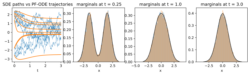
t=0.25: KS(SDE cloud, ODE cloud) = 0.0065
t=1.0: KS(SDE cloud, ODE cloud) = 0.0086
t=3.0: KS(SDE cloud, ODE cloud) = 0.0081
t=0.25: KS(SDE cloud, ODE cloud) = 0.0065
t=1.0: KS(SDE cloud, ODE cloud) = 0.0086
t=3.0: KS(SDE cloud, ODE cloud) = 0.0081
t=0.25: KS(SDE cloud, ODE cloud) = 0.0065
t=1.0: KS(SDE cloud, ODE cloud) = 0.0086
t=3.0: KS(SDE cloud, ODE cloud) = 0.0081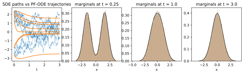
The leftmost panel contrasts the trajectories: thin blue SDE paths fluctuate and cross, while thick orange ODE trajectories are smooth and do not touch. Despite this difference, both histograms track the analytic marginal. The Kolmogorov–Smirnov distance between the two \(20{,}000\)-particle clouds stays in the \(0.006\)–\(0.009\) range. This empirical discrepancy includes finite-sample and numerical error; because the clouds share their initial sample, a standard independent-sample KS threshold is not the relevant calibration.
29.3.4 The Score Function
29.3.4.1 Definition and Geometry of the Score
The quantity
\[ \mathbf{s}_t(\mathbf{x}) = \nabla_{\mathbf{x}} \log p_t(\mathbf{x}) \tag{29.3.15}\]
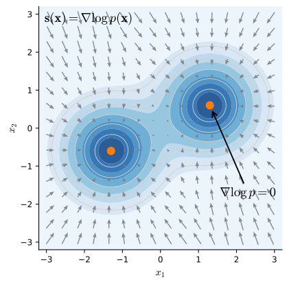
is called the score of the density \(p_t\) (in this context sometimes the Stein score). The gradient is with respect to the input \(\mathbf{x}\), not with respect to any parameters; this differs from the statistician’s score of Section 28.2.4.1, which is the canonical home of the definition and of the Fisher divergence built from it. Geometrically, \(\mathbf{s}_t\) is a vector field over data space: at each point it points in the direction of steepest ascent of the log-density (“uphill, toward the data”), with length proportional to how fast the density rises. It vanishes exactly at the interior critical points of \(p_t\): modes, troughs, and saddles. The Hessian, rather than the zero score alone, distinguishes these cases. Figure 29.3.2 shows the field for a two-mode density in two dimensions.
29.3.4.2 Two Worked Scores
The Gaussian. For \(p(\mathbf{x}) = \mathcal{N}(\mathbf{x}; \boldsymbol{\mu}, \sigma^2 I)\) the log-density is \(-\|\mathbf{x} - \boldsymbol{\mu}\|^2 / (2\sigma^2) + \textrm{const}\), so
\[ \nabla \log p(\mathbf{x}) = -\frac{\mathbf{x} - \boldsymbol{\mu}}{\sigma^2} : \tag{29.3.16}\]
a linear spring pulling toward the mean, stiffer for smaller \(\sigma\). (For a general covariance, \(-\Sigma^{-1}(\mathbf{x} - \boldsymbol{\mu})\).) This analytic score lets the numerical examples isolate solver error without also introducing estimation error.
The mixture. For \(p(x) = \sum_k \pi_k\, \mathcal{N}(x; \mu_k, s_k^2)\), differentiate \(\log p = \log \sum_k \pi_k N_k\) directly:
\[ \nabla \log p(x) = \frac{\sum_k \pi_k \nabla N_k}{\sum_j \pi_j N_j} = \sum_k \gamma_k(x) \left(-\frac{x - \mu_k}{s_k^2}\right), \qquad \gamma_k(x) = \frac{\pi_k N_k(x)}{\sum_j \pi_j N_j(x)}. \tag{29.3.17}\]
The mixture’s score is the responsibility-weighted average of the component scores: each point listens to all the springs, weighted by the posterior probability \(\gamma_k(x)\) that it belongs to component \(k\). (This posterior-average structure is no accident: it returns as the central identity behind denoising score matching in Section 29.4.) For the symmetric two-component case \(\pi_{1,2} = \tfrac12\), \(\mu_{1,2} = \pm\mu\), equal \(s_0^2\), the responsibilities collapse to a logistic and the score has a closed form:
\[ s(x) = \frac{\mu \tanh\!\left(\mu x / s_0^2\right) - x}{s_0^2}. \tag{29.3.18}\]
Near each mode, \(\tanh \to \pm 1\) and \(s(x) \approx -(x \mp \mu)/s_0^2\), the local Gaussian spring. At \(x = 0\) the score vanishes (the trough between the modes is a critical point too), but it is a repeller: infinitesimally to the right of \(0\) the score is large and positive, pushing mass toward \(+\mu\).
29.3.4.3 Independence from the Normalizing Constant
Consider a density known only up to its normalizing constant: \(p(\mathbf{x}) = \tilde{p}(\mathbf{x}) / Z\) with \(Z = \int \tilde{p}\, d\mathbf{x}\) unknown, the standing situation for energy-based models \(p \propto e^{-E(\mathbf{x})}\) (LeCun et al. 2006), where \(Z\) is an integral over all of \(\mathbb{R}^d\) that nobody can compute. The score does not care: since \(Z\) is constant in \(\mathbf{x}\), \(\nabla \log p = \nabla \log \tilde{p}\), the normalizer-blindness of the score Equation 28.2.13 established in Section 28.2.4.1. For the energy-based model the score is \(-\nabla E\). Score-based objectives can therefore avoid evaluating \(Z\). A neural network can represent a vector field without explicitly normalizing a density, and the Fisher divergence of Section 28.2.4.1 measures the quality of such a field directly. The probability-flow ODE and (next) the reverse SDE consume only the score. Estimating that field remains a statistical and computational problem, developed in Section 29.4.
The code makes all three points at once: it plots the bimodal score field 3, confirms the responsibility formula against it, locates the zeros, and checks that scaling the density by an arbitrary constant leaves the score unchanged.
gs = np.linspace(-3.5, 3.5, 1401)
dg = gs[1] - gs[0]
s_resp = score_t(gs, 0.0)                       # responsibility formula
s_tanh = (2.0 * np.tanh(2.0 * gs / 0.0625) - gs) / 0.0625   # closed form
print(f'max|responsibility - tanh form| = {np.abs(s_resp - s_tanh).max():.2e}')

zeros = gs[:-1][np.sign(s_resp[:-1]) != np.sign(s_resp[1:])]
print(f'score vanishes near: {np.unique(np.round(zeros, 2) + 0.0)}')

s_unnorm = np.gradient(np.log(7.3 * p_t(gs, 0.0)), dg)      # density scaled by 7.3
s_norm = np.gradient(np.log(p_t(gs, 0.0)), dg)
print(f'max|score(7.3 p) - score(p)| = {np.abs(s_unnorm - s_norm).max():.2e}')

dens = p_t(gs, 0.0)
d2l.plot(gs, [s_resp, dens * (np.abs(s_resp).max() / dens.max())], 'x', '',
legend=['score s(x)', 'density (rescaled)'], figsize=(5.5, 3))max|responsibility - tanh form| = 5.15e-14
score vanishes near: [-2. 0. 2.]
max|score(7.3 p) - score(p)| = 3.55e-13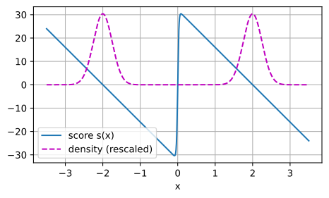
max|responsibility - tanh form| = 5.15e-14
score vanishes near: [-2.  0.  2.]
max|score(7.3 p) - score(p)| = 3.55e-13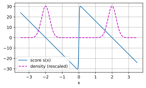
max|responsibility - tanh form| = 5.15e-14
score vanishes near: [-2.  0.  2.]
max|score(7.3 p) - score(p)| = 3.55e-13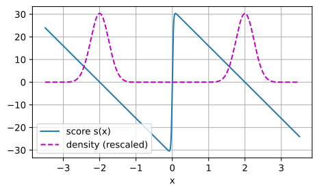
max|responsibility - tanh form| = 5.15e-14
score vanishes near: [-2.  0.  2.]
max|score(7.3 p) - score(p)| = 3.55e-13
The two formulas agree to machine precision; the zeros sit at the modes \(\pm 2\) and the repelling trough at \(0\); and multiplying the density by \(7.3\) moves the (finite-difference) score by less than \(10^{-12}\): the normalizer is invisible. The score is large near the low-density separation region where the log-density climbs steeply toward either mode; it also grows in the tails of this Gaussian mixture.
29.3.5 Time Reversal
29.3.5.1 Bayes on an Infinitesimal Step
The forward SDE destroys data into noise. Generation needs the process played backward, and the backward process is again a diffusion, with a drift we can write down. The intuition is one application of Bayes’ rule, on a single infinitesimal step.
Over a short interval \(\tau\), the forward kernel is the Euler–Maruyama Gaussian (Section 29.2.3.2):
\[ p(\mathbf{x}_{t+\tau} \mid \mathbf{x}_t) \approx \mathcal{N}\big(\mathbf{x}_{t+\tau};\; \mathbf{x}_t + \mathbf{f}(\mathbf{x}_t, t)\,\tau,\; g^2 \tau I\big). \]
For a reversed step, condition on the particle’s endpoint: \(\mathbf{x}_{t+\tau} = \mathbf{y}\), where did it come from? Bayes’ rule answers with the forward kernel reweighted by the marginal:
\[ p(\mathbf{x}_t = \mathbf{x} \mid \mathbf{x}_{t+\tau} = \mathbf{y}) \propto p(\mathbf{y} \mid \mathbf{x})\; p_t(\mathbf{x}). \]
Take logs and expand \(\log p_t(\mathbf{x})\) around the endpoint: \(\log p_t(\mathbf{x}) \approx \log p_t(\mathbf{y}) + (\mathbf{x} - \mathbf{y}) \cdot \nabla \log p_t(\mathbf{y})\), with corrections of higher order in \(\tau\) (the step is of size \(\sqrt{\tau}\)). Adding this linear term to the Gaussian exponent \(-\|\mathbf{x} - (\mathbf{y} - \mathbf{f}\tau)\|^2 / (2 g^2 \tau)\) and completing the square shifts the mean by \(g^2 \tau\, \nabla \log p_t(\mathbf{y})\):
\[ p(\mathbf{x} \mid \mathbf{y}) \approx \mathcal{N}\big(\mathbf{x};\; \mathbf{y} - [\mathbf{f}(\mathbf{y}, t) - g^2 \nabla \log p_t(\mathbf{y})]\,\tau,\; g^2 \tau I\big). \]
Stepping backward is therefore again a Gaussian kick of variance \(g^2 \tau\) (a diffusion) whose drift is the forward drift corrected by the full \(g^2\) times the score. The marginal \(p_t\) acts as a Bayesian prior that bends the reversed step toward where the data density actually was. (One bookkeeping remark for the careful reader: we evaluated \(\mathbf{f}\) and the score at the endpoint \(\mathbf{y}\) rather than at \(\mathbf{x}\); since the step itself is of size \(\sqrt{\tau}\), switching evaluation points perturbs the mean only at order \(\tau^{3/2}\), invisible at the order \(\tau\) we keep.)
29.3.5.2 Anderson’s Theorem
The infinitesimal picture is a theorem (Anderson 1982): the time-reversal of the diffusion \(d\mathbf{X} = \mathbf{f}\,dt + g\,d\mathbf{W}\) is the reverse-time SDE
\[ d\mathbf{X} = \big[\mathbf{f}(\mathbf{X}, t) - g(t)^2\, \nabla_{\mathbf{x}} \log p_t(\mathbf{X})\big]\,dt + g(t)\, d\bar{\mathbf{W}}, \tag{29.3.19}\]
integrated from \(t = T\) down to \(t = 0\), where \(\bar{\mathbf{W}}\) is a Brownian motion running in reverse time. Started from \(\mathbf{X}_T \sim p_T\), its marginals are \(p_t\) at every intermediate time: noise flows back into data.
Compare the drift corrections: the reverse SDE uses \(-g^2 \nabla \log p_t\), the probability-flow ODE used \(-\tfrac12 g^2 \nabla \log p_t\). The factor of two is real. To see why, and to prove Anderson’s theorem at the marginal level, use Fokker–Planck bookkeeping with a noise dial.
Proposition (one family, marginals fixed). Let \(p_t\) solve the Fokker–Planck equation. For any \(\lambda \ge 0\), the reverse-time SDE with noise scale \(\lambda g\) and drift
\[ \mathbf{b}_\lambda = \mathbf{f} - \tfrac{1 + \lambda^2}{2}\, g^2\, \nabla \log p_t \tag{29.3.20}\]
has marginals \(p_t\) when started from \(p_T\). The choice \(\lambda = 1\) is Anderson’s reverse SDE Equation 29.3.19; the choice \(\lambda = 0\) is the probability-flow ODE Equation 29.3.13.
Proof. Run the clock backward: let \(s = T - t\) and \(q_s = p_{T-s}\), the density evolution played in reverse, so \(\partial_s q_s = -\partial_t p_t = \nabla \cdot (\mathbf{f} p) - \tfrac12 g^2 \Delta p\). A reverse-time SDE \(d\mathbf{Y} = \mathbf{b}'\,ds + \lambda g\, d\mathbf{W}\) has its own Fokker–Planck equation \(\partial_s q = -\nabla \cdot (q\, \mathbf{b}') + \tfrac{\lambda^2}{2} g^2 \Delta q\). Matching the two right-hand sides and converting both Laplacians to transport form with Equation 29.3.11:
\[ -\nabla \cdot (q\, \mathbf{b}') = \nabla \cdot (\mathbf{f} q) - \tfrac{1 + \lambda^2}{2} g^2 \Delta q = \nabla \cdot \Big(q \Big[\mathbf{f} - \tfrac{1 + \lambda^2}{2} g^2 \nabla \log q\Big]\Big), \]
which holds with \(\mathbf{b}' = -\mathbf{f} + \tfrac{1+\lambda^2}{2} g^2 \nabla \log q\), the natural gradient-form choice. (Drifts with the same marginals can differ by a field that is divergence-free after multiplication by \(q\); in dimension \(d = 1\), and only there, decay at infinity forces that field to vanish, so the choice is unique.) Translating \(\mathbf{b}'\) back to forward-time notation flips its sign and gives Equation 29.3.20. It remains to pass from equal evolution equations plus the equal start \(q_0 = p_T\) to equal marginals: for \(\lambda = 0\) this is the transport-equation uniqueness used for the deterministic twin above, and for \(\lambda > 0\) it is uniqueness for a parabolic Fokker–Planck equation, which we take as a granted fact under our standing assumptions (Risken 1996). \(\blacksquare\)
The factor of two follows from the diffusion term in reverse time. The reverse process injects noise, which smooths its density. One \(-\tfrac12 g^2 \nabla \log p_t\) cancels the forward smoothing; this is the correction used by the probability-flow ODE, which injects no noise. A second \(-\tfrac12 g^2 \nabla \log p_t\) compensates for smoothing from the reverse-time noise. Anderson’s \(\lambda = 1\) includes both terms; intermediate values trade sampler stochasticity at fixed marginals, a freedom that diffusion-model samplers exploit deliberately (Section 29.4). Figure 29.3.3 shows the dial in action: three values of \(\lambda\), three path textures, one terminal histogram. Rigorously, Anderson’s result is a statement about the full reverse-time process (filtrations, reverse Brownian motions and all), stronger than the marginal statement proved here; see Anderson (1982) .
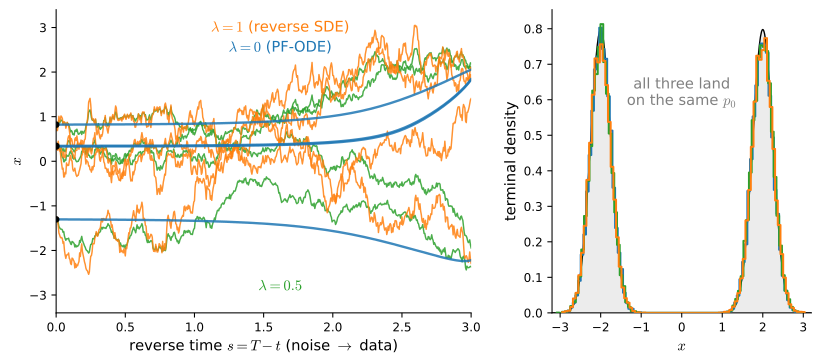
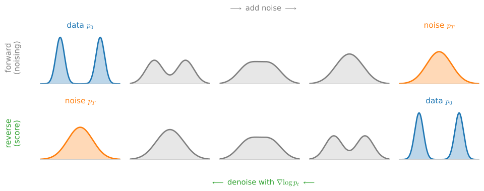
Equation Equation 29.3.19 separates known and unknown quantities. The forward drift \(\mathbf{f}\) and schedule \(g\): chosen by us. The terminal distribution \(p_T\): by design, approximately a known Gaussian (the whole point of noising). The score \(\nabla \log p_t\): the single unknown, the same one the probability-flow ODE needed. With the forward drift and schedule fixed, one estimated field can therefore be used by both samplers. Figure 29.3.4 shows the pair of processes as evolving densities, the one-dimensional counterpart of the two-dimensional example that Figure 29.4.2 tells in the next section.
29.3.5.3 Reverse-Time Sampling
The final demonstration is generation itself, with the learned network replaced by our closed-form mixture score: diffusion sampling with zero training. We draw \(20{,}000\) points from \(\mathcal{N}(0, 1)\) (which approximates \(p_T\) at \(T = 3\); the code measures how well) and integrate Anderson’s reverse SDE down to \(t = 0\) in the reversed clock \(s = T - t\), where Equation 29.3.19 reads \(d\mathbf{Y} = [-\mathbf{f} + g^2 \nabla \log p_t]\,ds + g\,d\mathbf{W}\).
gap = np.abs(p_t(gs, 3.0) - gauss(gs, 0.0, 1.0)).max()
print(f'max|p_T - N(0,1)| at T=3: {gap:.4f}  (vs peak {p_t(gs, 3.0).max():.4f})')

rng = np.random.default_rng(7)
n, T, steps = 20_000, 3.0, 600
dt = T / steps
x = rng.standard_normal(n)              # start from N(0,1), our stand-in for p_T
for k in range(steps):
    t = T - k * dt                      # current forward time, running down
    drift_rev = theta * x + sigma**2 * score_t(x, t)   # -f + g^2 * score
    x += drift_rev * dt + sigma * np.sqrt(dt) * rng.standard_normal(n)

left, right = x[x < 0], x[x >= 0]
print(f'mass split: {len(left)/n:.3f} / {len(right)/n:.3f}  (target 0.5 / 0.5)')
print(f'left mode:  mean {left.mean():+.3f}, std {left.std():.3f}  '
      f'(target -2.000, 0.250)')
print(f'right mode: mean {right.mean():+.3f}, std {right.std():.3f}  '
      f'(target +2.000, 0.250)')
print(f'KS(generated, exact p0 sample) = '
      f'{ks_distance(x, sample_p0(n, np.random.default_rng(99))):.4f}')

d2l.set_figsize((5.5, 3))
d2l.plt.hist(x, bins=80, density=True, alpha=0.4, color='C1',
             label='reverse-SDE samples')
d2l.plt.plot(gs, p_t(gs, 0.0), 'k', lw=1, label='data density $p_0$')
d2l.plt.xlabel('x'); d2l.plt.ylabel('density'); d2l.plt.legend();max|p_T - N(0,1)| at T=3: 0.0015 (vs peak 0.3974)
mass split: 0.500 / 0.500 (target 0.5 / 0.5)
left mode: mean -1.999, std 0.260 (target -2.000, 0.250)
right mode: mean +2.001, std 0.261 (target +2.000, 0.250)
KS(generated, exact p0 sample) = 0.0172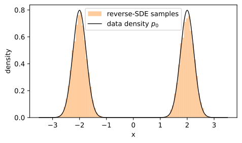
max|p_T - N(0,1)| at T=3: 0.0015  (vs peak 0.3974)
mass split: 0.500 / 0.500  (target 0.5 / 0.5)
left mode:  mean -1.999, std 0.260  (target -2.000, 0.250)
right mode: mean +2.001, std 0.261  (target +2.000, 0.250)
KS(generated, exact p0 sample) = 0.0172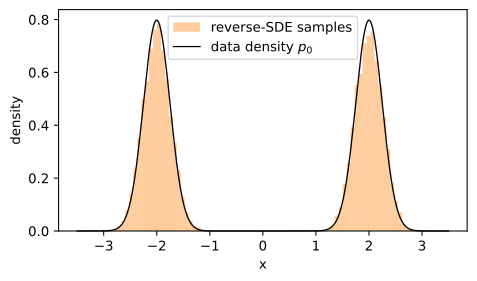
max|p_T - N(0,1)| at T=3: 0.0015  (vs peak 0.3974)
mass split: 0.500 / 0.500  (target 0.5 / 0.5)
left mode:  mean -1.999, std 0.260  (target -2.000, 0.250)
right mode: mean +2.001, std 0.261  (target +2.000, 0.250)
KS(generated, exact p0 sample) = 0.0172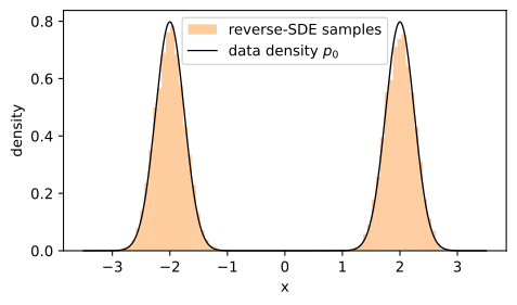
max|p_T - N(0,1)| at T=3: 0.0015  (vs peak 0.3974)
mass split: 0.500 / 0.500  (target 0.5 / 0.5)
left mode:  mean -1.999, std 0.260  (target -2.000, 0.250)
right mode: mean +2.001, std 0.261  (target +2.000, 0.250)
KS(generated, exact p0 sample) = 0.0172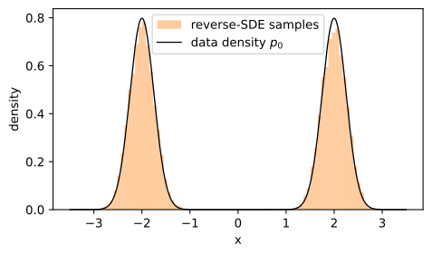
Starting from Gaussian reference noise (justified, since \(\max_x |p_T - \mathcal{N}(0,1)|\) is about \(0.0015\) against a density peak of \(0.40\)), the reverse SDE recovers modes at \(\pm 2.00\) and assigns mass \(0.500/0.500\) between them. The recovered mode widths read \(0.260\) and \(0.261\) against the target \(0.250\). Euler–Maruyama has \(O(\Delta t)\) weak bias under the conditions of Section 29.2.3.2, and a separate run with half the step gives widths \(0.255\) and \(0.252\). These finite experiments do not isolate discretization bias from Monte-Carlo variation or the small terminal-reference mismatch. Likewise, the Kolmogorov–Smirnov distance \(0.017\) to a fresh exact \(p_0\) sample is a sample statistic, not a universal noise floor. In a diffusion model, the analytic mixture score used here is replaced by a trained neural network, as developed in Section 29.4.
29.3.6 Summary
- A single SDE path is random, but the ensemble’s time-marginal \(p_t(\mathbf{x})\) evolves deterministically. Its law of motion is the Fokker–Planck equation. For diffusion matrix \(a=GG^\top\), it is \(\partial_t p=-\sum_i\partial_i(f_i p) +\tfrac12\sum_{ij}\partial_i\partial_j(a_{ij}p)\); the familiar scalar form uses \(a=g(t)^2I\). The probability current makes boundary assumptions explicit: reflecting boundaries have zero normal flux, periodic boundaries match flux, and absorbing boundaries can lose mass.
- Three vector-calculus facts are used: the divergence as flux per unit volume (with the divergence theorem), the Laplacian as deviation from the neighborhood average, and integration by parts \(\int h\, \nabla \cdot \mathbf{v} = -\int \nabla h \cdot \mathbf{v}\) for decaying fields.
- A Gaussian \(\mathcal{N}(m(t), v(t))\) solves the OU Fokker–Planck equation iff \(\dot m = -\theta m\) and \(\dot v = \sigma^2 - 2\theta v\), so the OU transition density solves it, and the stationary \(\mathcal{N}(0, \sigma^2/2\theta)\) is its steady state.
- Deterministic flows obey the continuity equation \(\partial_t p + \nabla \cdot (p \mathbf{v}) = 0\). Via \(\nabla p = p \nabla \log p\), the diffusion term can be written as transport: \(\tfrac12 g^2 \Delta p = \nabla \cdot (p \cdot \tfrac12 g^2 \nabla \log p)\), with a plus sign. So Fokker–Planck is a continuity equation with velocity \(\mathbf{v}_t = \mathbf{f} - \tfrac12 g^2 \nabla \log p_t\).
- The probability-flow ODE \(\dot{\mathbf{x}} = \mathbf{v}_t(\mathbf{x})\) shares every time-marginal with the SDE under the stated smoothness, positivity, boundary, and well-posedness assumptions. Its trajectories are deterministic and, where the flow exists uniquely in both directions, invertible. CNF likelihood evaluation is exact only with the exact field, divergence, and numerical integration.
- The score \(\nabla_{\mathbf{x}} \log p_t\) is a vector field pointing uphill on the log-density; it ignores the normalizing constant, so a score model need not evaluate a normalized density. Gaussian: \(-(\mathbf{x} - \boldsymbol{\mu})/\sigma^2\); mixtures: responsibility-weighted component scores.
- Anderson’s theorem: the time reversal of a diffusion is the diffusion \(d\mathbf{X} = [\mathbf{f} - g^2 \nabla \log p_t]\,dt + g\,d\bar{\mathbf{W}}\). The reverse SDE’s correction is \(g^2\) (it must undo forward smoothing and pre-compensate its own noise); the PF-ODE’s is \(\tfrac12 g^2\); a whole \(\lambda\)-family interpolates at fixed marginals. The score is the only unknown in all of them.
The probability-flow ODE, reverse SDE, and likelihood integral Equation 29.3.14 are used for sampling and likelihood evaluation in Section 29.4. Each requires the score.
29.3.7 Exercises
- Stationary distribution from scratch. Set \(\partial_t p = 0\) in the OU Fokker–Planck equation: \(0 = \theta\,\partial_x(x p) + \tfrac12 \sigma^2 \partial_{xx} p\). Integrate once in \(x\) and argue from decay at infinity that the constant of integration (the probability current) must vanish. Solve the resulting first-order ODE and confirm \(p_\infty = \mathcal{N}(0, \sigma^2/2\theta)\); no Gaussian ansatz allowed.
- Heat kernel. Use the moment-ODE proposition with \(\theta = 0\) to show that \(\mathcal{N}(x_0, v_0 + \sigma^2 t)\) solves the heat equation Equation 29.3.7, and conclude the marginal law of Brownian motion started from \(x_0\). What happens as \(v_0 \to 0\)?
- Continuity from conservation. Re-derive the continuity equation Equation 29.3.9 from the divergence theorem without looking, then derive the along-trajectory rule \(\frac{d}{dt} \log q_t(\mathbf{x}(t)) = -\nabla \cdot \mathbf{v}\) and reconcile it with the instantaneous change-of-variables formula of
- The sign, in \(d\) dimensions. Prove \(\tfrac12 \nabla \cdot (g^2 \nabla p) = \nabla \cdot (p \cdot \tfrac12 g^2 \nabla \log p)\) for \(\mathbf{x} \in \mathbb{R}^d\) and time-dependent scalar \(g\), stating exactly where you use \(p > 0\). Then explain, in one sentence each, why the right-hand side carries a plus sign while the probability-flow velocity carries \(-\tfrac12 g^2 \nabla \log p\).
- The Gaussian flow is affine. For OU started from the point mass \(\delta_{x_0}\), the marginal is the Gaussian
- Show that the probability-flow velocity \(v_t(x) = -\theta x - \tfrac12 \sigma^2 \cdot \big(-(x - m_t)/v_t\big)\) is affine in \(x\), solve the PF-ODE in closed form, and verify that it maps \(\mathcal{N}(m_s, v_s)\) to \(\mathcal{N}(m_t, v_t)\). Why can two of its trajectories never cross, while two SDE paths can?
- The factor of two. Re-derive the family Equation 29.3.20 from Fokker–Planck bookkeeping. Explain in words why the reverse SDE needs \(g^2 \nabla \log p_t\) where the PF-ODE needs only \(\tfrac12 g^2 \nabla \log p_t\), and what the dial \(\lambda\) trades off.
- Mixture scores. Derive the responsibility formula Equation 29.3.17 for \(K\) components, then specialize to the symmetric two-component case to obtain
- Find all zeros of 3 when \(\mu \gg s_0\) and classify each as a mode or a repeller of the ascent flow \(\dot x = s(x)\).
- Break the sampler. Rerun the reverse-SDE experiment with two modifications, one at a time: (a) an asymmetric prior \(\pi = (0.25, 0.75)\) (predict the recovered mass split before you run);
- the wrong drift correction \(\tfrac12 g^2 \nabla \log p_t\) while keeping the noise: describe what the recovered density looks like and explain why, using the \(\lambda\)-family with mismatched drift and noise.