%matplotlib inline
import numpy as np
from d2l import torch as d2l3.6 Generalization in Classification
The preceding sections fitted a softmax classifier by minimizing cross-entropy on a training set. The purpose of the fitted model is to classify new examples, so training accuracy alone is insufficient. A sufficiently expressive model can attain perfect training accuracy by memorizing the label associated with each distinct training input and returning that label whenever the same input appears again. And yet, memorizing the exact labels associated with the exact training examples does not tell us how to classify new examples. Memorization alone provides no rule for a genuinely new input.
This raises three questions:
- How many test examples do we need to give a good estimate of the accuracy of our classifiers on the underlying population?
- What happens if we keep evaluating models on the same test repeatedly?
- Why should we expect that fitting our linear models to the training set should fare any better than our naive memorization scheme?
Whereas Section 2.6 introduced overfitting and generalization in the context of linear regression, this section introduces foundational ideas of statistical learning theory. It turns out that we often can guarantee generalization a priori: for many models, and for any desired upper bound on the generalization gap \(t\), we can often determine some required number of samples \(n\) such that if our training set contains at least \(n\) samples, our empirical error will lie within \(t\) of the true error, for any data generating distribution. These guarantees provide important theoretical foundations but can be too loose to guide the sample sizes used for deep networks. In short, these guarantees suggest that ensuring generalization of deep neural networks a priori can require sample counts far beyond those used in practice (in some calculations, trillions or more), even when we find that, on the tasks we care about, deep neural networks typically generalize well with far fewer examples (thousands). Thus deep learning practitioners often forgo a priori guarantees altogether, instead employing methods that have generalized well on similar problems in the past, and certifying generalization post hoc through empirical evaluations. When we get to Section 4.5, we will revisit generalization and provide a light introduction to the vast scientific literature that has sprung in attempts to explain why deep neural networks generalize in practice.
3.6.1 The Test Set
Since we have already begun to rely on test sets to assess generalization error, we begin with the statistical properties of their estimates. Consider a fixed classifier \(f\), without worrying about how it was obtained. Moreover suppose that we possess a fresh dataset of examples \(\mathcal{D} = {(\mathbf{x}^{(i)},y^{(i)})}_{i=1}^n\) that were not used to train the classifier \(f\). The empirical error of our classifier \(f\) on \(\mathcal{D}\) is the fraction of instances for which the prediction \(f(\mathbf{x}^{(i)})\) disagrees with the true label \(y^{(i)}\), and is given by the following expression:
\[\epsilon_{\mathcal{D}}(f) = \frac{1}{n}\sum_{i=1}^n \mathbf{1}(f(\mathbf{x}^{(i)}) \neq y^{(i)}). \tag{3.6.1}\]
By contrast, the population error is the expected fraction of examples in the underlying population (some distribution \(P(X,Y)\) characterized by probability density function \(p(\mathbf{x},y)\)) for which our classifier disagrees with the true label:
\[\epsilon(f) = E_{(\mathbf{x}, y) \sim P} \mathbf{1}(f(\mathbf{x}) \neq y) = \int\int \mathbf{1}(f(\mathbf{x}) \neq y) p(\mathbf{x}, y) \;d\mathbf{x} dy. \tag{3.6.2}\]
While \(\epsilon(f)\) is the quantity that we actually care about, we cannot observe it directly, just as we cannot directly observe the average height in a large population without measuring every single person. We can only estimate this quantity based on samples. Because our test set \(\mathcal{D}\) is statistically representative of the underlying population, we can view \(\epsilon_{\mathcal{D}}(f)\) as a statistical estimator of the population error \(\epsilon(f)\). Moreover, because our quantity of interest \(\epsilon(f)\) is an expectation (of the random variable \(\mathbf{1}(f(X) \neq Y)\)) and the corresponding estimator \(\epsilon_{\mathcal{D}}(f)\) is the sample average, estimating the population error is the classical problem of mean estimation, which you may recall from Section 1.6.
An important classical result from probability theory called the central limit theorem guarantees, under its standard conditions, that for independent, identically distributed samples \(a_1, ..., a_n\) with finite mean \(\mu\) and finite standard deviation \(\sigma\), then, as the number of samples \(n\) approaches infinity, the sample average \(\hat{\mu}\) approximately tends towards a normal distribution centered at the true mean and with standard deviation \(\sigma/\sqrt{n}\). Consequently, as the number of examples grows large, our test error \(\epsilon_{\mathcal{D}}(f)\) should approach the true error \(\epsilon(f)\) at a rate of \(\mathcal{O}(1/\sqrt{n})\). Thus, to estimate our test error twice as precisely, we must collect four times as large a test set. To shrink the uncertainty in our estimate a hundredfold, we must collect ten thousand times as large a test set. (Note that more test data never reduces the error itself, only our uncertainty about its value.) In general, such a rate of \(\mathcal{O}(1/\sqrt{n})\) is often the best we can hope for in statistics.
Now that we know something about the asymptotic rate at which our test error \(\epsilon_{\mathcal{D}}(f)\) converges to the true error \(\epsilon(f)\), we can zoom in on some important details. Recall that the random variable of interest \(\mathbf{1}(f(X) \neq Y)\) can only take values \(0\) and \(1\) and thus is a Bernoulli random variable, characterized by a parameter indicating the probability that it takes value \(1\). Here, \(1\) means that our classifier made an error, so the parameter of our random variable is actually the true error rate \(\epsilon(f)\). The variance \(\sigma^2\) of a Bernoulli depends on its parameter (here, \(\epsilon(f)\)) according to the expression \(\epsilon(f)(1-\epsilon(f))\). This function is largest when the true error rate is close to \(0.5\) and can be far lower when it is close to \(0\) or close to \(1\). This tells us that the asymptotic standard deviation of our estimate \(\epsilon_{\mathcal{D}}(f)\) of the error \(\epsilon(f)\) (over the choice of the \(n\) test samples) cannot be any greater than \(\sqrt{0.25/n}\).
If we ignore the fact that this rate characterizes behavior as the test set size approaches infinity rather than when we possess finite samples, this tells us that if we want our test error \(\epsilon_{\mathcal{D}}(f)\) to approximate the population error \(\epsilon(f)\) such that one standard deviation corresponds to an interval of \(\pm 0.01\), then we should collect roughly 2500 samples. If we want to fit two standard deviations in that range and thus be 95% confident that \(\epsilon_{\mathcal{D}}(f) \in \epsilon(f) \pm 0.01\), then we will need 10,000 samples!
This turns out to be the size of the test sets for many popular benchmarks in machine learning. Improvements of \(0.01\) or less should therefore be interpreted together with the test-set size and uncertainty of the estimate. Of course, when the error rates are much closer to \(0\), then an improvement of \(0.01\) can indeed be a big deal.
The preceding analysis is asymptotic: i.e., how the relationship between \(\epsilon_{\mathcal{D}}\) and \(\epsilon\) evolves as our sample size goes to infinity. Because the random variable is bounded, we can also obtain finite-sample bounds by applying an inequality due to Hoeffding (1963), proved in Section 27.6:
\[P\left(|\epsilon_{\mathcal{D}}(f) - \epsilon(f)| \geq t\right) < 2\exp\left( - 2n t^2 \right). \tag{3.6.3}\]
Solving for the smallest dataset size that would allow us to conclude with 95% confidence that the distance \(t\) between our estimate \(\epsilon_{\mathcal{D}}(f)\) and the true error rate \(\epsilon(f)\) does not exceed \(0.01\), you will find that roughly 18,500 examples are required, as compared with the 10,000 examples suggested by the asymptotic analysis above. If you go deeper into statistics you will find that this trend holds generally. Finite-sample guarantees are typically more conservative. The comparable order of magnitude here also shows why asymptotic calculations can provide useful approximations even when they are not finite-sample guarantees.
All of the above is pencil-and-paper reasoning, but it is also one short simulation away from being visible. Fix a classifier whose true error is \(\epsilon(f) = 0.1\) and draw many hypothetical test sets: each per-example indicator is a Bernoulli\((0.1)\) coin, so a size-\(n\) test set produces an estimate \(\epsilon_{\mathcal{D}}(f) \sim \mathrm{Binomial}(n, 0.1)/n\).
%matplotlib inline
import numpy as np
from d2l import tensorflow as d2l%matplotlib inline
import numpy as np
from d2l import jax as d2l%matplotlib inline
import numpy as np
from d2l import mxnet as d2lWe simulate 1000 such test sets at each size \(n\), record the empirical spread (standard deviation) of the resulting error estimates, and compare it with the two envelopes derived above: the CLT prediction \(\sqrt{\epsilon(1-\epsilon)/n}\) and the 95% Hoeffding radius \(\sqrt{\log(2/0.05)/(2n)}\).
rng = np.random.default_rng(0)
eps, trials = 0.1, 1000
ns = np.array([100, 300, 1000, 3000, 10000])
spread = np.array([(rng.binomial(n, eps, trials) / n).std() for n in ns])
clt = np.sqrt(eps * (1 - eps) / ns)           # CLT standard deviation
hoeff = np.sqrt(np.log(2 / 0.05) / (2 * ns))  # 95% Hoeffding radius
d2l.plot(ns, [spread, clt, hoeff], 'test set size n', 'spread of the estimate',
         legend=['simulated sd', 'CLT sd', 'Hoeffding 95% radius'],
         xscale='log', yscale='log')


On log–log axes all three curves are parallel lines of slope \(-\frac{1}{2}\): the \(\sqrt{n}\) law made visible. The simulated spread sits right on top of the CLT prediction, but the two envelopes are not measured on the same footing: the CLT curve is one standard deviation, while the Hoeffding curve is a two-sided 95% radius. Converting the CLT curve to its own 95% radius (\(1.96\sigma\)) closes most of the gap; the Hoeffding radius still runs about \(2.3\times\) above it, which is the price of a bound valid at every finite \(n\) rather than only asymptotically.
3.6.2 Test Set Reuse
The guarantee above applies to a classifier fixed independently of the test set. Reusing one test set creates two distinct problems. First, evaluating \(k\) prespecified classifiers introduces multiplicity: even when every reported interval has 95% coverage on its own, the probability that at least one interval misses its target grows with \(k\). Simultaneous guarantees must account for this collection of comparisons.
Second, model development is usually adaptive. If \(f_2\) is selected after observing the test performance of \(f_1\), then \(f_2\) is no longer independent of the test set. Repeated feedback can therefore overfit the holdout itself, a phenomenon called adaptive overfitting (Dwork et al. 2015). A validation set should absorb model selection and hyperparameter tuning, while the test set is reserved for a small number of final evaluations. Reports should disclose the number and adaptivity of comparisons; long-running benchmarks should periodically replace their hidden test data.
How bad can it get? A simulation makes the false-discovery half of the problem concrete in its purest form. Take one binary test set of \(n = 1000\) examples and evaluate \(k\) “classifiers” that ignore the inputs entirely and guess labels uniformly at random, so that every one of them has true accuracy exactly \(0.5\). We track the best test accuracy seen so far as \(k\) grows:
n, k = 1000, 10000
labels = rng.integers(0, 2, n)                 # one fixed test set
guesses = rng.integers(0, 2, (k, n))           # k random-guess classifiers
best = np.maximum.accumulate((guesses == labels).mean(axis=1))
d2l.plot(np.arange(1, k + 1), best, 'number of models evaluated',
         'best test accuracy so far', xscale='log')


The best apparent accuracy climbs steadily, exceeding \(0.56\) after ten thousand tries, even though the classifiers contain no learned signal: the models are coin flips, and the climb is pure selection, growing like \(\sqrt{\log(k)/(2n)}\) by the same Hoeffding bound applied to \(k\) events at once. Whenever you pick the best of many models by their score on one shared test set, some of the apparent improvement is exactly this effect; and an adaptive modeler can climb faster still, steering each new model toward what scored well before.
3.6.3 Statistical Learning Theory
A test set provides a post hoc estimate for a particular trained classifier. It does not, by itself, explain why a learning procedure should generalize or how much data a model class requires. Statistical learning theory addresses the complementary, a priori question. Its bounds relate the generalization gap to properties of the hypothesis class, the learning rule, and the sample size.
Learning theorists aim to bound the difference between the empirical error \(\epsilon_{\mathcal{S}}(f_{\mathcal{S}})\) of a learned classifier \(f_{\mathcal{S}}\), both trained and evaluated on the training set \(\mathcal{S}\), and the true error \(\epsilon(f_{\mathcal{S}})\) of that same classifier on the underlying population. This might look similar to the evaluation problem that we just addressed but there is a major difference. Earlier, the classifier \(f\) was fixed and we only needed a dataset for evaluative purposes. And indeed, any fixed classifier does generalize: its error on a (previously unseen) dataset is an unbiased estimate of the population error. But what can we say when a classifier is trained and evaluated on the same dataset? Can we ever be confident that the training error will be close to the testing error?
Suppose that our learned classifier \(f_{\mathcal{S}}\) must be chosen from some pre-specified set of functions \(\mathcal{F}\). Recall from our discussion of test sets that while it is easy to estimate the error of a single classifier, collections of classifiers require simultaneous control. Even if the empirical error of any one (fixed) classifier will be close to its true error with high probability, once we consider a collection of classifiers, we need to worry about the possibility that just one of them will receive a badly estimated error. The worry is that we might pick such a classifier and thereby grossly underestimate the population error. Moreover, even for linear models, because their parameters are continuously valued, we are typically choosing from an infinite class of functions (\(|\mathcal{F}| = \infty\)).
One ambitious solution to the problem is to develop analytic tools for proving uniform convergence, i.e., that with high probability, the empirical error rate for every classifier in the class \(f\in\mathcal{F}\) will simultaneously converge to its true error rate. In other words, we seek a theoretical principle that would allow us to state that with probability at least \(1-\delta\) (for some small \(\delta\)) no classifier’s error rate \(\epsilon(f)\) (among all classifiers in the class \(\mathcal{F}\)) will be misestimated by more than some small amount \(\alpha\). Clearly, we cannot make such statements for all model classes \(\mathcal{F}\). Recall the class of memorization machines that always achieve empirical error \(0\) but never outperform random guessing on the underlying population.
In a sense the class of memorizers is too flexible. No such uniform convergence result could possibly hold. On the other hand, a fixed classifier is useless: it generalizes perfectly, but fits neither the training data nor the test data. The central question of learning has thus historically been framed as a trade-off between more flexible (higher variance) model classes that better fit the training data but risk overfitting, versus more rigid (higher bias) model classes that generalize well but risk underfitting. A central question in learning theory has been to develop the appropriate mathematical analysis to quantify where a model sits along this spectrum, and to provide the associated guarantees.
In a series of papers, Vapnik and Chervonenkis extended the theory on the convergence of relative frequencies to more general classes of functions (Vapnik and Chervonenkis 1964, 1968, 1971, 1981, 1991; Vapnik and Chervonenkis 1974). One of the key contributions of this line of work is the Vapnik–Chervonenkis (VC) dimension, which measures (one notion of) the complexity (flexibility) of a model class. Moreover, one of their key results bounds the difference between the empirical error and the population error as a function of the VC dimension and the number of samples:
\[P\left(\epsilon(f_{\mathcal{S}}) - \epsilon_{\mathcal{S}}(f_{\mathcal{S}}) < \alpha\right) \geq 1-\delta \ \textrm{ for }\ \alpha \geq c \sqrt{(\textrm{VC} - \log \delta)/n}. \tag{3.6.4}\]
Here \(\delta > 0\) is the probability that the bound is violated, \(\alpha\) is the upper bound on the generalization gap, and \(n\) is the dataset size. Lastly, \(c > 0\) is a constant that depends only on the scale of the loss that can be incurred. One use of the bound might be to plug in desired values of \(\delta\) and \(\alpha\) to determine how many samples to collect. A class shatters a set of points if, for every possible \(\pm\) labeling of them, some model \(f\) in the class agrees with that labeling. The VC dimension is the largest number of points the class can shatter. For example, linear models on \(d\)-dimensional inputs have VC dimension \(d+1\). As Figure 3.6.1 illustrates, a line in the plane can realize every labeling of three points in general position, while no line can realize the XOR labeling of four points, which already shows that lines cannot shatter these four points. Radon’s theorem below supplies the general upper bound, and hence a VC dimension of exactly \(3\) for two-dimensional linear classifiers (matching \(d+1\) with \(d=2\)). The general statement holds in both directions, and neither is deep. For the lower bound, the \(d+1\) points \(\{\mathbf{0}, \mathbf{e}_1, \ldots, \mathbf{e}_d\}\) can be shattered by weights constructed directly from the desired labels; exercise 5 walks you through it. For the upper bound, no set of \(d+2\) points can be shattered: by Radon’s theorem (Radon 1921), any \(d+2\) points in \(\mathbb{R}^d\) can be partitioned into two subsets whose convex hulls intersect, and no halfspace can put two intersecting hulls on opposite sides.
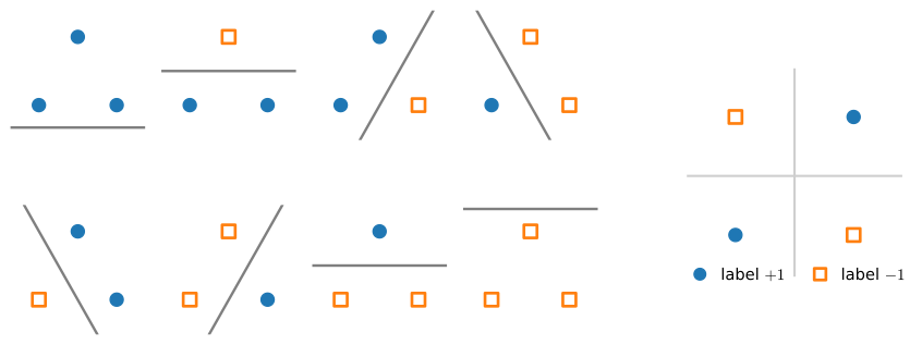
For complex models, the resulting bound is often pessimistic and obtaining this guarantee typically requires far more examples than are actually needed to achieve the desired error rate. Note also that fixing the model class and \(\delta\), our error rate again decays with the usual \(\mathcal{O}(1/\sqrt{n})\) rate. It seems unlikely that we could do better in terms of \(n\). However, as we vary the model class, VC dimension can present a pessimistic picture of the generalization gap.
3.6.4 Summary
The most straightforward way to evaluate a model is to consult a test set comprised of previously unseen data. Test set evaluations provide an unbiased estimate of the true error and converge at the desired \(\mathcal{O}(1/\sqrt{n})\) rate as the test set grows. We can provide approximate confidence intervals based on exact asymptotic distributions or valid finite sample confidence intervals based on (more conservative) finite sample guarantees. Test set evaluation is central to modern machine learning research. However, test sets are seldom true test sets (used by multiple researchers again and again). Once the same test set is used to evaluate multiple models, controlling for false discovery can be difficult. This can cause huge problems in theory. In practice, the significance of the problem depends on the size of the holdout sets in question and whether they are merely being used to choose hyperparameters or if they are leaking information more directly. Nevertheless, it is good practice to curate real test sets (or multiple) and to be as conservative as possible about how often they are used.
Hoping to provide a more satisfying solution, statistical learning theorists have developed methods for guaranteeing uniform convergence over a model class. If indeed every model’s empirical error simultaneously converges to its true error, then we are free to choose the model that performs best, minimizing the training error, knowing that it too will perform similarly well on the holdout data. Crucially, any one of such results must depend on some property of the model class. Vladimir Vapnik and Alexey Chervonenkis introduced the VC dimension, presenting uniform convergence results that hold for all models in a VC class. The training errors for all models in the class are (simultaneously) guaranteed to be close to their true errors, and guaranteed to grow even closer at \(\mathcal{O}(1/\sqrt{n})\) rates. Following the discovery of VC dimension, numerous alternative complexity measures have been proposed, each facilitating an analogous generalization guarantee. One such measure, Rademacher complexity, is developed in full in Section 27.6, which also reproduces from scratch (as double descent) the empirical behavior of overparameterized models that we are about to describe. See Boucheron et al. (2005) for a detailed discussion of several advanced ways of measuring function complexity. These complexity measures are broadly useful in statistical theory, but their direct application does not explain why deep neural networks generalize (Zhang et al. 2021). Deep neural networks often have millions of parameters (or more), and can easily assign random labels to large collections of points. Nevertheless, they generalize well on practical problems and on some tasks they generalize better when they are larger and deeper, despite incurring higher VC dimensions. We revisit generalization in the context of deep learning in Section 4.5.
3.6.5 Exercises
- If we wish to estimate the error of a fixed model \(f\) to within \(0.0001\) with probability greater than 99.9%, how many samples do we need?
- Suppose that somebody else possesses a labeled test set \(\mathcal{D}\) and only makes available the unlabeled inputs (features). Now suppose that you can only access the test set labels by running a model \(f\) (with no restrictions placed on the model class) on each of the unlabeled inputs and receiving the corresponding error \(\epsilon_{\mathcal{D}}(f)\). How many models would you need to evaluate before you leak the entire test set and thus could appear to have error \(0\), regardless of your true error?
- What is the VC dimension of the class of fifth-order polynomials?
- What is the VC dimension of axis-aligned rectangles on two-dimensional data?
- Prove the lower bound VC \(\geq d+1\) for linear classifiers \(f(\mathbf{x}) = \operatorname{sign}(\mathbf{w}^\top \mathbf{x} + b)\) on \(\mathbb{R}^d\) by shattering the \(d+1\) points \(\{\mathbf{0}, \mathbf{e}_1, \ldots, \mathbf{e}_d\}\) (the origin and the standard unit vectors). Given any desired labels \(\sigma_0, \sigma_1, \ldots, \sigma_d \in \{\pm 1\}\), set \(b = \sigma_0 / 2\) and read the weights off the labels as \(w_i = \sigma_i - b\). Verify that \(f(\mathbf{0}) = \sigma_0\) and \(f(\mathbf{e}_i) = \sigma_i\) for every \(i\). Combined with the Radon argument in the text for the upper bound, this proves VC \(= d+1\) exactly.
- In Figure 3.6.1 the three shattered points are in general position (not collinear). Show that three collinear points can not be shattered by halfplanes: which labeling is unrealizable? Explain why this does not contradict the VC dimension of lines in the plane being \(3\). (Hint: the VC dimension asks whether some set of a given size can be shattered, not whether every set can.)