%matplotlib inline
from d2l import torch as d2l
import torch
from torch import nn16.1 Generative Adversarial Networks
The generative models introduced so far were trained by likelihood: evaluate the probability of the observed data and adjust the parameters to increase it. This procedure requires a model whose probabilities can be evaluated. It therefore excludes a direct neural sampler that transforms random noise into data in a single forward pass but provides no tractable density for its output.
Generative adversarial networks (Goodfellow et al. 2014) train such samplers through comparison rather than likelihood. A second network, the discriminator, learns to distinguish generated samples from real data. The generator then receives gradients through the discriminator and learns to make this classification difficult. As the generator improves, the discriminator must detect increasingly subtle differences between the two distributions. When the generated distribution matches the data distribution, the best discriminator cannot identify a sample’s source more reliably than a random guess. The original paper described this interaction through the analogy of a counterfeiter and a police force. The same principle underlies several fast samplers, tokenizers, and vocoders discussed at the end of this chapter.
This interaction raises a precise question: which discrepancy between distributions does the original GAN objective minimize? An optimal discriminator computes the pointwise log ratio between the data and generator densities. Substituting this discriminator into the objective yields a divergence that vanishes exactly when the two distributions match. The analysis also identifies a weakness of the original generator loss: confidently rejected samples receive the smallest gradients. A non-saturating generator loss corrects this weighting and provides stronger gradients for those samples.
%matplotlib inline
from d2l import jax as d2l
import jax
from jax import numpy as jnp
from flax import nnx
import numpy as np
import optax
16.1.1 From Likelihood to Comparison
Maximum likelihood is distribution matching. Fitting a density \(p_\theta\) to samples maximizes \(\sum_i \log p_\theta(x_i)\), and Section 27.3.2.1 showed that this is the same as minimizing the Kullback–Leibler divergence from the empirical distribution to the model. When the likelihood is intractable rather than absent, as in latent-variable models, the ELBO of Section 27.3.5 substitutes a bound. Either way, training needs \(\log p_\theta(x)\) or a surrogate for it.
The models of this chapter offer neither. An implicit generator draws a latent variable \(z \sim \mathcal{N}(0, I_k)\) and outputs \(x' = G(z)\), where \(G\) is a neural network. Sampling is a single forward pass. The distribution of \(x'\) is the pushforward of the Gaussian through \(G\), but its density is generally unavailable. When \(k\) is smaller than the data dimension, the samples concentrate on a lower-dimensional surface and have no density with respect to volume in the ambient space. Even when the dimensions match, evaluating the density would require an invertible \(G\) with a tractable Jacobian. An unrestricted neural sampler therefore does not provide the quantity required by maximum likelihood.
One possible response is to restrict \(G\) until its likelihood becomes tractable. Such a restriction is useful only if likelihood reliably measures sample quality. Consider a model that mixes the data density with noise,
\[ \tilde p \;=\; 0.01\, p_{\textrm{data}} + 0.99\, p_{\textrm{noise}}. \]
For every \(x\) we have \(\tilde p(x) \geq 0.01\, p_{\textrm{data}}(x)\), so \(\log \tilde p(x) \geq \log p_{\textrm{data}}(x) - \log 100\). The expected log-likelihood of \(\tilde p\) is therefore within \(\log 100 \approx 4.6\) nats of the best achievable by any model. For images or audio, whose log-likelihoods can contain thousands of nats, this penalty is small. Yet 99 percent of the mixture’s samples are noise. A model can thus have nearly optimal likelihood while remaining useless as a sampler (Theis et al. 2016). Evaluating a sampler requires examining its samples.
Statistics provides a direct way to compare samples. Given real and generated examples, a two-sample test asks whether the two sets came from the same distribution. A generative adversarial network turns this test into a training signal: fit a classifier, called the discriminator, to distinguish generated data from real data, and train the generator to make that classification difficult. Relative to the chosen discriminator class, the generator has matched the data when no discriminator can reliably separate their samples. Figure 16.1.1 shows the resulting computation.
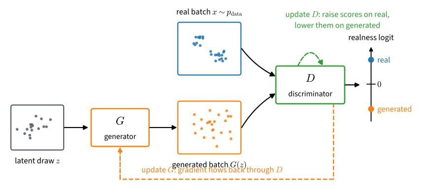
The diagram specifies the training mechanism but not the quantity being optimized. We compute the objective at the discriminator’s best response, then determine whether the resulting generator gradient is useful. Both calculations use the original logistic loss.
16.1.2 The Log-Loss Game
The discriminator solves a binary classification problem. Draw a label \(y \sim \textrm{Bernoulli}(\tfrac12)\). If \(y = 1\), draw \(x\) from the data density \(p\); if \(y = 0\), draw \(x\) from the generator density \(q\). The marginal density of \(x\) is the balanced mixture \(m = (p + q)/2\), which describes a sample whose source is unknown. Throughout this chapter, \(p\) denotes the data distribution and \(q\) the generator distribution. Two derived quantities will recur: the density ratio \(\rho = p/q\) and its logarithm \(\lambda = \log \rho\). The discriminator is a function \(D: \mathcal{X} \to \mathbb{R}\) that produces a realness logit. With \(\sigma(t) = 1/(1 + e^{-t})\), the value \(\sigma(D(x))\) estimates \(P(y = 1 \mid x)\), and a larger \(D(x)\) indicates stronger evidence that \(x\) came from the data. We will repeatedly use the identities \(\sigma(-t) = 1 - \sigma(t)\) and \(\tfrac{d}{dt} \log \sigma(t) = \sigma(-t)\).
The natural loss for a probabilistic classifier is the log loss, and on the balanced problem the discriminator’s expected negative log-likelihood is \(-\tfrac12 E_{x \sim p}[\log \sigma(D(x))] - \tfrac12 E_{x' \sim q}[\log \sigma(-D(x'))]\). Dropping the factor \(\tfrac12\) and flipping the sign gives the objective the discriminator maximizes,
\[ V(D) \;=\; E_{x \sim p}\big[\log \sigma(D(x))\big] + E_{x' \sim q}\big[\log \sigma(-D(x'))\big], \tag{16.1.1}\]
the value function of Goodfellow et al. (2014). The first term increases when the discriminator assigns high probabilities to real samples, and the second increases when it assigns low probabilities to generated samples. Since both terms are expectations of log-probabilities, \(V(D) \leq 0\). The generator minimizes \(V\) and influences only the second term, so training solves the minimax problem \(\min_G \max_D V\). Maximizing \(V\) is equivalent to minimizing the classifier’s negative log-likelihood. The best achievable value therefore measures how well \(p\) and \(q\) can be distinguished, which gives the objective its information-theoretic interpretation.
16.1.2.1 The Optimal Critic
The maximization over \(D\) looks like a problem in function space, but it separates into independent scalar problems. The integrand of Equation 16.1.1 at a point \(x\) is \(p(x) \log \sigma(D(x)) + q(x) \log \sigma(-D(x))\), which depends on \(D\) only through the single number \(D(x)\). Writing \(s = \sigma(D(x)) \in (0, 1)\), the problem at each point is to maximize \(p \log s + q \log(1 - s)\), a strictly concave function of \(s\) whose stationarity condition \(p/s = q/(1-s)\) has the unique solution
\[ \sigma(D^\star(x)) = \frac{p(x)}{p(x) + q(x)} = P(y = 1 \mid x), \qquad D^\star(x) = \log \frac{p(x)}{q(x)} = \lambda(x). \tag{16.1.2}\]
The optimal discriminator returns the Bayes posterior for the labeling problem, and its logit is the log density ratio. This pointwise argument assumes that both densities are positive. Where one density vanishes, the optimal logit is infinite and is attained only in the limit; the corresponding divergences are interpreted as extended-real quantities throughout the chapter. Although \(q\) has no computable density, Equation 16.1.2 shows that a classifier can estimate the function of \(q\) required by the objective. An unconstrained critic trained with log loss is therefore a density-ratio estimator. Other losses and critic classes will produce related estimates later in the chapter. The objective also determines the additive constant: shifting \(D^\star\) by any \(b \neq 0\) strictly decreases \(V\) (Exercise 1). Pairwise critics will provide a contrasting case in which such shifts leave the objective unchanged.
16.1.2.2 The Value of the Game
Substituting the best response into the objective identifies the discrepancy minimized by the generator. With \(\sigma(D^\star) = p/(p+q) = p/(2m)\) and \(\sigma(-D^\star) = q/(2m)\),
\[ V(D^\star) = \int p \log \frac{p}{2m} + \int q \log \frac{q}{2m} = \mathrm{KL}(p \,\|\, m) + \mathrm{KL}(q \,\|\, m) - 2 \log 2 . \]
The two divergences are exactly the ones that define the Jensen–Shannon divergence of Equation 28.2.2, \(\mathrm{JS}(p, q) = \tfrac12 \mathrm{KL}(p \| m) + \tfrac12 \mathrm{KL}(q \| m)\), so
\[ \max_D V(D) = 2\,\mathrm{JS}(p, q) - 2 \log 2 . \tag{16.1.3}\]
Against an optimal discriminator, minimizing \(V\) therefore minimizes the Jensen–Shannon divergence between the generator and the data. This divergence vanishes exactly when \(q = p\), so the minimax objective has the desired fixed point. Equivalently, the discriminator’s minimum negative log-likelihood is \(\log 2 - \mathrm{JS}(p, q)\), the chance-level loss minus the divergence. The experiment below compares this prediction with the observed training loss.
Two rewritings of \(\mathrm{JS}\) explain what kind of quantity the game has produced. Expanding each Kullback–Leibler term as \(\mathrm{KL}(p \| m) = -H[p] - \int p \log m\) and collecting the mixture terms into \(\int m \log m = -H[m]\) gives
\[ \mathrm{JS}(p, q) \;=\; H[m] - \frac{H[p] + H[q]}{2}, \tag{16.1.4}\]
where \(H\) denotes differential entropy. The first term is the uncertainty of a sample whose source is unknown; the second is the average uncertainty conditional on its source. Their difference measures the uncertainty attributable to the unknown source. Because entropy is strictly concave, this Jensen gap is nonnegative and vanishes only when \(p = q\). Mixing distinct distributions increases uncertainty relative to the average entropy of the components.
The labeled-mixture setup gives a second interpretation. Let \(y\) be the Bernoulli source label and \(x \sim m\) the sample. Their mutual information is \(I(x; y) = H[x] - H[x \mid y]\), whose two terms coincide with those in Equation 16.1.4. Hence \(\mathrm{JS}(p, q) = I(x; y)\): the divergence measures how many nats a sample provides about its source. Accordingly, the optimal classifier’s loss \(\log 2 - I(x; y)\) improves on a random guess by this amount. The divergence is \(\mathrm{JS}\), whereas the value of the game is \(2\,\mathrm{JS} - 2\log 2\).
The mutual-information interpretation also provides bounds. Since \(I(x; y) = H(y) - H(y \mid x)\), a binary source label carries at most one bit: \(I(x; y) \leq H(y) = \log 2\). Equality holds exactly when \(x\) determines \(y\), which occurs when the supports of \(p\) and \(q\) are disjoint and every sample identifies its source. Together with nonnegativity,
\[ 0 \;\leq\; \mathrm{JS}(p, q) \;\leq\; \log 2 . \]
Section 28.2 derived the same bounds from the Kullback–Leibler form, including the case of disjoint supports. Once the two supports separate, the divergence remains at \(\log 2\) regardless of the distance between them. The experiment below demonstrates the resulting loss of gradient.
16.1.3 The Generator’s Gradient
The generator influences only the second term of Equation 16.1.1, so playing the minimax game literally means minimizing \(E_z[\log \sigma(-D(G(z)))]\) over the generator’s parameters \(\theta\), with the discriminator held fixed. Differentiating through \(x' = G(z)\) with the identity \(\tfrac{d}{du} \log \sigma(-u) = -\sigma(u)\) gives
\[ \nabla_\theta \, E_z\big[\log \sigma(-D(G(z)))\big] = -\,E_z\big[\sigma(D(x'))\, \nabla_\theta D(G(z))\big] , \]
where \(\nabla_\theta D(G(z))\) is the gradient of the composite map. The contribution from each generated sample points in the direction that increases its critic score. For sample \(x'\), this contribution is weighted by \(\sigma(D(x'))\), the discriminator’s estimated probability that the sample is real. Early in training, or for a poorly modeled sample later on, the discriminator may have \(D(x') \ll 0\). The weight \(\sigma(D(x'))\) is then exponentially small. The loss has saturated: samples that the discriminator rejects most confidently contribute least to the generator update.
Goodfellow et al. (2014) therefore substitute a different generator loss in practice: rather than minimizing the probability of being called fake, the generator maximizes the probability of being called real, minimizing \(-E_z[\log \sigma(D(G(z)))]\). The same differentiation, now with \(\tfrac{d}{du} \log \sigma(u) = \sigma(-u)\), gives
\[ \nabla_\theta \Big({-E_z\big[\log \sigma(D(G(z)))\big]}\Big) = -\,E_z\big[\sigma(-D(x'))\, \nabla_\theta D(G(z))\big] . \]
The two losses generate the same update direction \(\nabla_\theta D\) per sample and differ only in the weight attached to it:
\[ w_{\textrm{sat}}(x') = \sigma(D(x')), \qquad w_{\textrm{ns}}(x') = \sigma(-D(x')) = 1 - \sigma(D(x')). \tag{16.1.5}\]
The non-saturating weight \(w_{\textrm{ns}}\) is near one where the saturating weight is near zero. A confidently rejected sample therefore contributes substantially to the non-saturating update.
Swapping the weighting does not change the population minimizer against an optimal critic. Substituting the optimal critic \(D^\star = \lambda\) into the non-saturating loss and using \(\sigma(\lambda) = p/(2m)\),
\[ -E_{x' \sim q}\big[\log \sigma(\lambda(x'))\big] = \log 2 + \mathrm{KL}(q \,\|\, p) - \mathrm{KL}(q \,\|\, m) \;\geq\; \log 2 + \tfrac12\, \mathrm{KL}(q \,\|\, p), \tag{16.1.6}\]
The inequality follows from the convexity of \(\mathrm{KL}(q \,\|\, \cdot)\) and the fact that \(m\) is the midpoint of \(p\) and \(q\): \(\mathrm{KL}(q \| m) \leq \tfrac12 \mathrm{KL}(q \| p) + \tfrac12 \mathrm{KL}(q \| q)\), where the final term is zero. The bound exceeds \(\log 2\) unless \(\mathrm{KL}(q \| p) = 0\), and the loss equals \(\log 2\) at \(q = p\). Thus, with an optimal critic, the non-saturating loss is minimized uniquely at \(q = p\). It reweights the gradient field without changing the desired solution. Although its value differs from \(\mathrm{JS}\), both objectives have the unique minimizer \(q=p\). The following experiment examines when this reweighting helps and when it remains insufficient.
16.1.4 Fitting a Gaussian
The analysis makes three predictions. At the fixed point, the discriminator’s per-sample loss equals \(\log 2 \approx 0.693\). Away from the fixed point, a trained critic approximates the log density ratio \(\lambda = \log(p/q)\). Finally, because the two generator losses weight samples oppositely, a confidently rejected generator should continue learning with the non-saturating loss but stall with the saturating loss. A two-dimensional Gaussian permits all three predictions to be checked against closed forms: when the data are Gaussian and the generator is linear, \(p\), \(q\), and \(\lambda\) are available exactly.
16.1.4.1 Data and Models
The data are a standard Gaussian pushed through a fixed linear map: \(x = z A + b\) with \(z \sim \mathcal{N}(0, I_2)\), giving \(p = \mathcal{N}(b, A^\top A)\). The chosen \(A\) makes the cloud a thin tilted ellipse rather than a round blob, so matching it requires learning an orientation and two very different scales. Training works from a fixed sample of one thousand draws, while the analytic comparisons below use the population densities.
torch.manual_seed(0)
Z = torch.normal(0.0, 1.0, (1000, 2))
A = torch.tensor([[1.0, 2.0], [-0.1, 0.5]])
b = torch.tensor([1.0, 2.0])
data = Z @ A + b
d2l.set_figsize()
d2l.plt.scatter(data[:100, 0], data[:100, 1], s=8);
print(f'covariance of the data distribution:\n{A.T @ A}')
covariance of the data distribution:
tensor([[1.0100, 1.9500],
[1.9500, 4.2500]])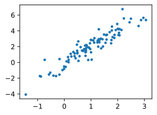
Z = jax.random.normal(jax.random.PRNGKey(0), (1000, 2))
A = jnp.array([[1.0, 2.0], [-0.1, 0.5]])
b = jnp.array([1.0, 2.0])
data = Z @ A + b
d2l.set_figsize()
d2l.plt.scatter(data[:100, 0], data[:100, 1], s=8);
print(f'covariance of the data distribution:\n{A.T @ A}')
covariance of the data distribution:
[[1.01 1.95]
[1.95 4.25]]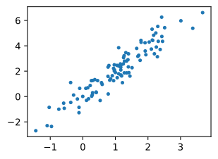
The generator is a single linear layer, so its output distribution is Gaussian and its mean and covariance can be recovered from the weights. This choice makes the verification below exact. The discriminator is a small multilayer perceptron with two tanh hidden layers. It is flexible enough to score points in the plane but has no access to the closed-form densities used in our analysis. A factory function builds both networks from a fixed seed so that later cells can restart from the same initialization.
def make_nets():
    torch.manual_seed(7)
    net_G = nn.Sequential(nn.Linear(2, 2))
    net_D = nn.Sequential(nn.Linear(2, 5), nn.Tanh(),
                          nn.Linear(5, 3), nn.Tanh(),
                          nn.Linear(3, 1))
    for net in (net_G, net_D):
        for w in net.parameters():
            nn.init.normal_(w, 0, 0.02)
    return net_G, net_D
class Generator(nnx.Module):
def __init__(self, rngs):
normal = nnx.initializers.normal(0.02)
self.out = nnx.Linear(2, 2, kernel_init=normal, bias_init=normal,
rngs=rngs)
def __call__(self, x):
return self.out(x)
class Discriminator(nnx.Module):
def __init__(self, rngs):
normal = nnx.initializers.normal(0.02)
self.h1 = nnx.Linear(2, 5, kernel_init=normal, bias_init=normal,
rngs=rngs)
self.h2 = nnx.Linear(5, 3, kernel_init=normal, bias_init=normal,
rngs=rngs)
self.out = nnx.Linear(3, 1, kernel_init=normal, bias_init=normal,
rngs=rngs)
def __call__(self, x):
return self.out(nnx.tanh(self.h2(nnx.tanh(self.h1(x)))))
def make_nets():
return Generator(nnx.Rngs(7)), Discriminator(nnx.Rngs(8))16.1.4.2 The Update Rules
One training iteration is two half-steps, one per player. The discriminator update ascends Equation 16.1.1 on a minibatch, implemented as logistic regression with label one for data and zero for generated samples; the generator’s parameters are held fixed during this half-step. Both update functions are saved to the d2l library, since Section 16.5 trains image networks with the identical rules.
def update_D(X, Z, net_D, net_G, loss, trainer_D):
    """Update the discriminator."""
    batch_size = X.shape[0]
    ones = torch.ones((batch_size,), device=X.device)
    zeros = torch.zeros((batch_size,), device=X.device)
    trainer_D.zero_grad()
    real_Y = net_D(X)
    # The generator is the fixed player here: detach its output
    fake_X = net_G(Z)
    fake_Y = net_D(fake_X.detach())
    loss_D = (loss(real_Y, ones.reshape(real_Y.shape)) +
              loss(fake_Y, zeros.reshape(fake_Y.shape))) / 2
    loss_D.backward()
    trainer_D.step()
    return loss_D
@nnx.jit
def update_D(X, Z, net_D, net_G, optimizer_D):
    """Update the discriminator."""
    batch_size = X.shape[0]
    fake_X = net_G(Z)  # computed outside the loss: no gradient to net_G
    def loss_D_fn(model_D):
        real_Y = model_D(X).squeeze()
        fake_Y = model_D(fake_X).squeeze()
        return (jnp.sum(optax.sigmoid_binary_cross_entropy(
                    real_Y, jnp.ones(batch_size))) +
                jnp.sum(optax.sigmoid_binary_cross_entropy(
                    fake_Y, jnp.zeros(batch_size)))) / 2
    loss_D, grads_D = nnx.value_and_grad(loss_D_fn)(net_D)
    optimizer_D.update(net_D, grads_D)
    return loss_D
The generator update implements the non-saturating loss of Equation 16.1.5: generated samples are fed to the discriminator under the label one, so that the resulting cross-entropy is \(-E[\log \sigma(D(G(z)))]\). The discriminator has changed since its half-step, so its scores are recomputed rather than reused. In the JAX version, the loss closure takes both models as explicit arguments and differentiates only with respect to the first; this keeps the update rule reusable for networks whose forward pass mutates state, which the convolutional models of Section 16.5 require.
def update_G(Z, net_D, net_G, loss, trainer_G):
    """Update the generator on the non-saturating loss."""
    batch_size = Z.shape[0]
    ones = torch.ones((batch_size,), device=Z.device)
    trainer_G.zero_grad()
    # net_D changed in its half-step, so recompute the scores
    fake_Y = net_D(net_G(Z))
    loss_G = loss(fake_Y, ones.reshape(fake_Y.shape))
    loss_G.backward()
    trainer_G.step()
    return loss_G
@nnx.jit
def update_G(Z, net_D, net_G, optimizer_G):
    """Update the generator on the non-saturating loss."""
    def loss_G_fn(model_G, model_D):
        fake_Y = model_D(model_G(Z)).squeeze()
        return jnp.sum(optax.sigmoid_binary_cross_entropy(
            fake_Y, jnp.ones(Z.shape[0])))
    loss_G, grads_G = nnx.value_and_grad(loss_G_fn, argnums=0)(net_G, net_D)
    optimizer_G.update(net_G, grads_G)
    return loss_G
16.1.4.3 Training
The loop alternates the two half-steps over minibatches, records each player’s per-sample loss, and stores generated samples at selected epochs. These snapshots are used by the comparison experiment below. Adam serves as the optimizer for both players, with the discriminator given the larger learning rate so that its scores stay close to their best response to the current generator.
def train(net_D, net_G, data_iter, num_epochs, lr_D=0.05, lr_G=0.005,
          step_G=None, snapshot_epochs=()):
    step_G = step_G if step_G is not None else update_G
    loss = nn.BCEWithLogitsLoss(reduction='sum')
    trainer_D = torch.optim.Adam(net_D.parameters(), lr=lr_D)
    trainer_G = torch.optim.Adam(net_G.parameters(), lr=lr_G)
    history, snapshots = [], {}
    for epoch in range(1, num_epochs + 1):
        metric = d2l.Accumulator(3)
        for (X,) in data_iter:
            Zb = torch.normal(0, 1, (X.shape[0], 2))
            metric.add(
                update_D(X, Zb, net_D, net_G, loss, trainer_D).detach(),
                step_G(Zb, net_D, net_G, loss, trainer_G).detach(),
                X.shape[0])
        history.append((metric[0] / metric[2], metric[1] / metric[2]))
        if epoch in snapshot_epochs:
            with torch.no_grad():
                snapshots[epoch] = net_G(torch.normal(0, 1, (200, 2)))
    return torch.tensor(history), snapshots
def train(net_D, net_G, data_iter, num_epochs, lr_D=0.05, lr_G=0.005,
step_G=None, snapshot_epochs=(), seed=1):
step_G = step_G if step_G is not None else update_G
key = jax.random.PRNGKey(seed)
optimizer_D = nnx.Optimizer(net_D, optax.adam(lr_D), wrt=nnx.Param)
optimizer_G = nnx.Optimizer(net_G, optax.adam(lr_G), wrt=nnx.Param)
history, snapshots = [], {}
for epoch in range(1, num_epochs + 1):
loss_D_sum, loss_G_sum, n = 0.0, 0.0, 0
for (X,) in data_iter:
key, subkey = jax.random.split(key)
Zb = jax.random.normal(subkey, (X.shape[0], 2))
loss_D_sum += update_D(X, Zb, net_D, net_G, optimizer_D)
loss_G_sum += step_G(Zb, net_D, net_G, optimizer_G)
n += X.shape[0]
history.append((loss_D_sum / n, loss_G_sum / n))
if epoch in snapshot_epochs:
key, subkey = jax.random.split(key)
snapshots[epoch] = net_G(jax.random.normal(subkey, (200, 2)))
return np.array(history), snapshotsTwenty epochs suffice for the default run. The left panel below tracks both losses; the right panel overlays generated samples on the data.
data_iter = d2l.load_array((data,), batch_size=8)
net_G, net_D = make_nets()
history, _ = train(net_D, net_G, data_iter, num_epochs=20)
with torch.no_grad():
    fake = net_G(torch.normal(0, 1, (200, 2)))
fig, axes = d2l.plt.subplots(1, 2, figsize=(9, 3.2))
axes[0].plot(range(1, 21), history[:, 0], label='discriminator')
axes[0].plot(range(1, 21), history[:, 1], label='generator')
axes[0].axhline(0.693, ls='--', c='gray', lw=1)
axes[0].set_xlabel('epoch'), axes[0].set_ylabel('per-sample loss')
axes[0].legend()
axes[1].scatter(data[:100, 0], data[:100, 1], s=8, label='real')
axes[1].scatter(fake[:100, 0], fake[:100, 1], s=8, label='generated')
axes[1].legend()
fig.tight_layout()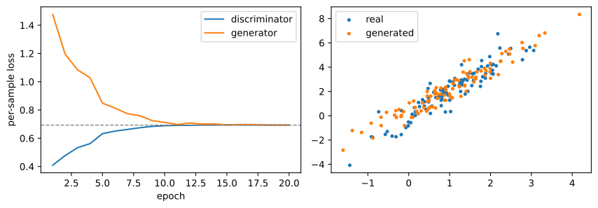
np.random.seed(0)
data_iter = d2l.load_array((np.asarray(data),), batch_size=8)
net_G, net_D = make_nets()
history, _ = train(net_D, net_G, data_iter, num_epochs=20)
key = jax.random.PRNGKey(4)
fake = net_G(jax.random.normal(key, (200, 2)))
fig, axes = d2l.plt.subplots(1, 2, figsize=(9, 3.2))
axes[0].plot(range(1, 21), history[:, 0], label='discriminator')
axes[0].plot(range(1, 21), history[:, 1], label='generator')
axes[0].axhline(0.693, ls='--', c='gray', lw=1)
axes[0].set_xlabel('epoch'), axes[0].set_ylabel('per-sample loss')
axes[0].legend()
axes[1].scatter(data[:100, 0], data[:100, 1], s=8, label='real')
axes[1].scatter(fake[:100, 0], fake[:100, 1], s=8, label='generated')
axes[1].legend()
fig.tight_layout()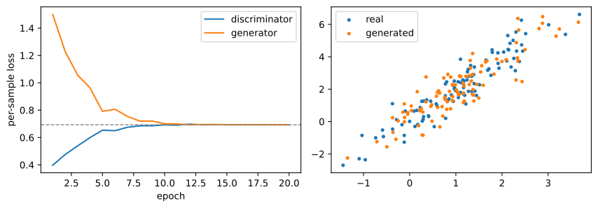
The loss curves provide an empirical check of the value calculation. While real and generated samples remain distinguishable, the discriminator loss is below \(\log 2\). As the generator improves, the loss approaches the dashed line at \(\log 2 \approx 0.693\). Equation Equation 16.1.3 places the optimal discriminator’s per-sample negative log-likelihood at \(\log 2 - \mathrm{JS}(p, q)\), so the observed rise is consistent with \(\mathrm{JS}\) approaching zero. The generator loss approaches the same level from above for a different reason. By Equation 16.1.6, the non-saturating loss against a near-optimal critic approaches its minimum \(\log 2\) as \(q\) approaches \(p\). The sample overlay provides a separate qualitative check: generated samples occupy the same tilted ellipse as the data. Nevertheless, a discriminator loss of \(\log 2\) establishes only that the trained discriminator cannot distinguish the samples. It does not prove that \(q=p\), so the next two measurements evaluate the fit independently.
16.1.4.4 Verifying the Optimal Critic
Equation Equation 16.1.2 states that an optimal critic computes \(\lambda = \log(p/q)\). Both densities are known in this experiment: \(p = \mathcal{N}(b, A^\top A)\) by construction, and the trained linear generator determines the Gaussian \(q\). Two conditions are needed for a useful check. First, the theorem concerns the best response to a fixed generator, whereas ordinary training alternates between the two networks. We therefore freeze the generator and give the critic additional steps to converge. Second, by the end of the main run \(q\) is so close to \(p\) that \(\lambda\) is nearly zero throughout the sampled region. We instead freeze the partially trained generator at epoch ten, when the mismatch remains measurable.
def gaussian_logpdf(x, mu, Sigma):
    diff = x - mu
    sol = torch.linalg.solve(Sigma, diff.T).T
    return -0.5 * ((diff * sol).sum(1)
                   + torch.logdet(2 * torch.pi * Sigma))

def generator_gaussian(net_G):
    W, c = net_G[0].weight.detach(), net_G[0].bias.detach()
    return c, W @ W.T

net_G_mid, net_D_mid = make_nets()
train(net_D_mid, net_G_mid, data_iter, num_epochs=10)
loss = nn.BCEWithLogitsLoss(reduction='sum')
trainer_D = torch.optim.Adam(net_D_mid.parameters(), lr=0.01)
torch.manual_seed(2)
for _ in range(2000):  # critic-only steps against the frozen generator
    X = data[torch.randint(0, 1000, (256,))]
    Zb = torch.normal(0, 1, (256, 2))
    update_D(X, Zb, net_D_mid, net_G_mid, loss, trainer_D)
def gaussian_logpdf(x, mu, Sigma):
diff = x - mu
sol = jnp.linalg.solve(Sigma, diff.T).T
return -0.5 * ((diff * sol).sum(1)
+ jnp.linalg.slogdet(2 * jnp.pi * Sigma)[1])
def generator_gaussian(net_G):
K, c = net_G.out.kernel[...], net_G.out.bias[...]
return c, K.T @ K
np.random.seed(2)
data_iter_v = d2l.load_array((np.asarray(data),), batch_size=8)
net_G_mid, net_D_mid = make_nets()
train(net_D_mid, net_G_mid, data_iter_v, num_epochs=10)
optimizer_D = nnx.Optimizer(net_D_mid, optax.adam(0.01), wrt=nnx.Param)
key = jax.random.PRNGKey(2)
for _ in range(2000): # critic-only steps against the frozen generator
key, k1, k2 = jax.random.split(key, 3)
X = data[jax.random.randint(k1, (256,), 0, 1000)]
Zb = jax.random.normal(k2, (256, 2))
update_D(X, Zb, net_D_mid, net_G_mid, optimizer_D)The comparison uses samples from the mixture: two hundred real and two hundred generated. The two Gaussian densities give the analytic value of \(\lambda\), while a forward pass gives the critic estimate.
mu_q, Sigma_q = generator_gaussian(net_G_mid)
with torch.no_grad():
    xs = torch.cat([data[:200], net_G_mid(torch.normal(0, 1, (200, 2)))])
    lam = (gaussian_logpdf(xs, b, A.T @ A)
           - gaussian_logpdf(xs, mu_q, Sigma_q))
    D_out = net_D_mid(xs).squeeze()
print(f'correlation(D, lambda) = '
      f'{torch.corrcoef(torch.stack([lam, D_out]))[0, 1]:.3f}')
print(f'mean |D - lambda| = {(D_out - lam).abs().mean():.3f} nats')
d2l.set_figsize((4.2, 3.4))
d2l.plt.scatter(lam, D_out, s=8)
lims = [float(lam.min()), float(lam.max())]
d2l.plt.plot(lims, lims, 'k--', lw=1)
d2l.plt.xlabel(r'analytic $\log(p/q)$')
d2l.plt.ylabel('critic output')
correlation(D, lambda) = 0.868
mean |D - lambda| = 0.157 natsText(0, 0.5, 'critic output')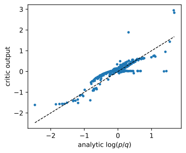
mu_q, Sigma_q = generator_gaussian(net_G_mid)
key, subkey = jax.random.split(key)
xs = jnp.concatenate([data[:200],
                      net_G_mid(jax.random.normal(subkey, (200, 2)))])
lam = (gaussian_logpdf(xs, b, A.T @ A)
       - gaussian_logpdf(xs, mu_q, Sigma_q))
D_out = net_D_mid(xs).squeeze()
print(f'correlation(D, lambda) = '
      f'{jnp.corrcoef(jnp.stack([lam, D_out]))[0, 1]:.3f}')
print(f'mean |D - lambda| = {jnp.abs(D_out - lam).mean():.3f} nats')
d2l.set_figsize((4.2, 3.4))
d2l.plt.scatter(lam, D_out, s=8)
lims = [float(lam.min()), float(lam.max())]
d2l.plt.plot(lims, lims, 'k--', lw=1)
d2l.plt.xlabel(r'analytic $\log(p/q)$')
d2l.plt.ylabel('critic output')
correlation(D, lambda) = 0.949
mean |D - lambda| = 0.154 natsText(0, 0.5, 'critic output')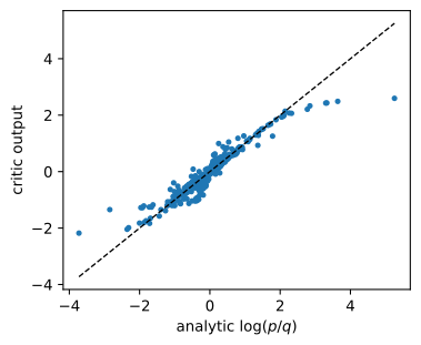
The points lie close to the dashed identity line. As Equation 16.1.2 predicts, a three-layer network trained only for classification has learned the log density ratio, with a mean error well below one nat. The errors increase at extreme values of \(\lambda\), where one density is nearly zero and the mixture supplies few samples. The objective constrains the critic only where \(m\) places appreciable mass; elsewhere the network extrapolates (Exercise 5 maps this error over the plane). Density-ratio estimation is therefore least accurate where the ratio is most extreme, a limitation examined further in the next section.
16.1.4.5 Quantifying the Fit
The sample overlay lets the fit be judged by eye; the linear generator lets it be measured in nats. For Gaussians in \(d\) dimensions the Kullback–Leibler divergence has the closed form (Kullback 1959)
\[ \mathrm{KL}\big(\mathcal{N}(\mu_0, \Sigma_0) \,\|\, \mathcal{N}(\mu_1, \Sigma_1)\big) = \tfrac12 \Big[ \operatorname{tr}(\Sigma_1^{-1} \Sigma_0) + (\mu_1 - \mu_0)^\top \Sigma_1^{-1} (\mu_1 - \mu_0) - d + \log \tfrac{\det \Sigma_1}{\det \Sigma_0} \Big], \tag{16.1.7}\]
the multivariate form of the univariate formula derived in Equation 28.1.5. We report \(\mathrm{KL}(q \,\|\, p)\), the direction that charges the generator for placing mass where the data has little, evaluated at initialization and after training.
def kl_gaussians(mu0, S0, mu1, S1):
    diff = mu1 - mu0
    return 0.5 * (torch.trace(torch.linalg.solve(S1, S0))
                  + diff @ torch.linalg.solve(S1, diff) - len(mu0)
                  + torch.logdet(S1) - torch.logdet(S0))

mu_p, Sigma_p = b, A.T @ A
for name, net in [('at initialization', make_nets()[0]),
                  ('after training   ', net_G)]:
    mu_q, Sigma_q = generator_gaussian(net)
    print(f'KL(q || p) {name}: '
          f'{kl_gaussians(mu_q, Sigma_q, mu_p, Sigma_p):.3f} nats')
KL(q || p) at initialization: 8.694 nats
KL(q || p) after training : 0.128 natsdef kl_gaussians(mu0, S0, mu1, S1):
diff = mu1 - mu0
return 0.5 * (jnp.trace(jnp.linalg.solve(S1, S0))
+ diff @ jnp.linalg.solve(S1, diff) - len(mu0)
+ jnp.linalg.slogdet(S1)[1] - jnp.linalg.slogdet(S0)[1])
mu_p, Sigma_p = b, A.T @ A
for name, net in [('at initialization', make_nets()[0]),
('after training ', net_G)]:
mu_q, Sigma_q = generator_gaussian(net)
print(f'KL(q || p) {name}: '
f'{kl_gaussians(mu_q, Sigma_q, mu_p, Sigma_p):.3f} nats')KL(q || p) at initialization: 7.856 nats
KL(q || p) after training : 0.051 natsThe divergence falls from roughly eight nats at initialization to a small fraction of a nat. Although the training loop never evaluates the generator density, the classifier supplies enough information to fit its parameters. The resulting generator distribution closely approximates the data distribution.
16.1.4.6 Saturating versus Non-Saturating Training
Testing the two weights in Equation 16.1.5 requires an initialization at which they differ substantially. In the preceding run, the initial generator emits samples near the origin, about one standard deviation from the data mean. The critic never becomes confident enough to drive \(w_{\textrm{sat}}\) toward zero, and both losses train successfully. We therefore initialize the generator’s bias far from the data, where the critic can reject its samples confidently. Two runs begin from this same initialization and differ only in the sign that produces the saturating or non-saturating weight.
def update_G_saturating(Z, net_D, net_G, loss, trainer_G):
    batch_size = Z.shape[0]
    zeros = torch.zeros((batch_size,), device=Z.device)
    trainer_G.zero_grad()
    fake_Y = net_D(net_G(Z))
    # minimize E[log sigma(-D)]: the minimax game taken literally
    loss_G = -loss(fake_Y, zeros.reshape(fake_Y.shape))
    loss_G.backward()
    trainer_G.step()
    return loss_G

runs = {}
for name, step in [('non-saturating', update_G),
                   ('saturating', update_G_saturating)]:
    net_G_ab, net_D_ab = make_nets()
    with torch.no_grad():
        net_G_ab[0].bias += torch.tensor([-6.0, 6.0])
    torch.manual_seed(1)
    hist, snaps = train(net_D_ab, net_G_ab, data_iter, num_epochs=30,
                        lr_G=0.01, step_G=step, snapshot_epochs=(10, 30))
    runs[name] = (hist, snaps)
    mu_q, Sigma_q = generator_gaussian(net_G_ab)
    print(f'{name}: final KL(q || p) = '
          f'{kl_gaussians(mu_q, Sigma_q, mu_p, Sigma_p):.2f} nats')
non-saturating: final KL(q || p) = 1.03 nats
saturating: final KL(q || p) = 326.99 nats@nnx.jit
def update_G_saturating(Z, net_D, net_G, optimizer_G):
def loss_G_fn(model_G, model_D):
fake_Y = model_D(model_G(Z)).squeeze()
# minimize E[log sigma(-D)]: the minimax game taken literally
return -jnp.sum(optax.sigmoid_binary_cross_entropy(
fake_Y, jnp.zeros(Z.shape[0])))
loss_G, grads_G = nnx.value_and_grad(loss_G_fn, argnums=0)(net_G, net_D)
optimizer_G.update(net_G, grads_G)
return loss_G
runs = {}
for name, step in [('non-saturating', update_G),
('saturating', update_G_saturating)]:
net_G_ab, net_D_ab = make_nets()
net_G_ab.out.bias[...] += jnp.array([-6.0, 6.0])
np.random.seed(9) # reseed per arm: identical minibatch streams
data_iter_ab = d2l.load_array((np.asarray(data),), batch_size=8)
hist, snaps = train(net_D_ab, net_G_ab, data_iter_ab, num_epochs=30,
lr_G=0.01, step_G=step, snapshot_epochs=(10, 30),
seed=9)
runs[name] = (hist, snaps)
mu_q, Sigma_q = generator_gaussian(net_G_ab)
print(f'{name}: final KL(q || p) = '
f'{kl_gaussians(mu_q, Sigma_q, mu_p, Sigma_p):.2f} nats')non-saturating: final KL(q || p) = 77.73 nats
saturating: final KL(q || p) = 323.85 natsThe panels below show each run’s samples partway through and at the end of the budget, over the data in grey, together with both discriminator loss traces.
fig, axes = d2l.plt.subplots(1, 3, figsize=(10.5, 3.2))
for ax, (name, (hist, snaps)) in zip(axes[:2], runs.items()):
    ax.scatter(data[:150, 0], data[:150, 1], s=6, c='lightgray',
               label='real')
    ax.scatter(snaps[10][:, 0], snaps[10][:, 1], s=6, label='epoch 10')
    ax.scatter(snaps[30][:, 0], snaps[30][:, 1], s=6, label='epoch 30')
    ax.set_xlim(-8, 6), ax.set_ylim(-6, 8)
    ax.set_title(name), ax.legend()
for name, (hist, snaps) in runs.items():
    axes[2].plot(range(1, 31), hist[:, 0], label=name)
axes[2].axhline(0.693, ls='--', c='gray', lw=1)
axes[2].set_xlabel('epoch'), axes[2].set_ylabel('discriminator loss')
axes[2].legend()
fig.tight_layout()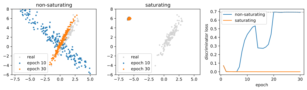
fig, axes = d2l.plt.subplots(1, 3, figsize=(10.5, 3.2))
for ax, (name, (hist, snaps)) in zip(axes[:2], runs.items()):
    ax.scatter(data[:150, 0], data[:150, 1], s=6, c='lightgray',
               label='real')
    ax.scatter(snaps[10][:, 0], snaps[10][:, 1], s=6, label='epoch 10')
    ax.scatter(snaps[30][:, 0], snaps[30][:, 1], s=6, label='epoch 30')
    ax.set_xlim(-8, 6), ax.set_ylim(-6, 8)
    ax.set_title(name), ax.legend()
for name, (hist, snaps) in runs.items():
    axes[2].plot(range(1, 31), hist[:, 0], label=name)
axes[2].axhline(0.693, ls='--', c='gray', lw=1)
axes[2].set_xlabel('epoch'), axes[2].set_ylabel('discriminator loss')
axes[2].legend()
fig.tight_layout()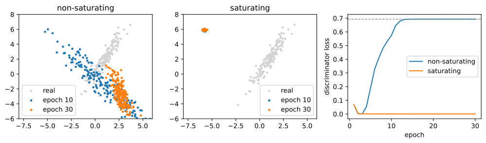
The printed KL values quantify the predicted difference. In both frameworks, the saturating generator remains near its initialization and its final divergence exceeds three hundred nats. The discriminator reaches near-zero loss within the first few epochs, so \(\sigma(D(x')) \approx 0\) for every generated sample. Equation Equation 16.1.5 then assigns nearly zero weight to each generator update. Because the generator scarcely changes, the discriminator can continue to reject its samples confidently.
The non-saturating loss reduces the divergence by orders of magnitude, although the result within this budget depends on the random draw. The stored PyTorch run reaches the data region and ends near one nat; as the distributions approach, the discriminator loss returns to \(\log 2\). The stored JAX run makes partial progress and ends at several dozen nats because the small critic provides an imperfect score surface. The reweighting provides a useful gradient under confident rejection, but it does not guarantee a complete fit within a fixed training budget.
Reweighting helps only when the critic’s score surface retains a useful slope. Both weights in Equation 16.1.5 multiply the same factor \(\nabla_\theta D\), so the non-saturating loss can amplify this factor but cannot create it. In this experiment, the small tanh critic was far from its best response, and its smooth score surface supplied a gradient. An optimal critic on separated supports supplies no such gradient.
Consider the smallest example: two point masses \(p = \delta_0\) and \(q_\theta = \delta_\theta\) on the line. For every \(\theta \neq 0\), their supports are disjoint, \(\mathrm{JS}(p,q_\theta) = \log 2\), and the value of the game is independent of \(\theta\). A constant objective supplies no gradient with respect to \(\theta\), regardless of how its samples are reweighted, even when the generator lies arbitrarily close to the solution.
The same issue arises in high dimensions. A generator maps a lower-dimensional latent variable into the sample space, so generated samples often concentrate near a low-dimensional set whose support is nearly disjoint from that of the data (Arjovsky and Bottou 2017). The next section compares adversarial discrepancies according to whether they preserve a gradient when supports separate.
16.1.5 Summary
An implicit generator supplies samples without a tractable density, so maximum likelihood cannot be applied directly. The mixture example also shows that a high likelihood need not imply useful samples. Adversarial training instead learns a comparison between real and generated data.
For the logistic loss, pointwise optimization gives \(\sigma(D^\star) = p/(p+q)\) and \(D^\star = \lambda = \log(p/q)\). Substituting this critic into the value function yields \(2\,\mathrm{JS}(p,q) - 2\log 2\). The Jensen–Shannon divergence is both the Jensen gap of entropy at the equal mixture and the mutual information \(I(x;y)\) between a sample and its origin. This information interpretation gives the upper bound \(\log 2\), attained when the supports are disjoint.
The saturating and non-saturating generator losses have the same fixed point but weight samples by \(\sigma(D)\) and \(\sigma(-D)\), respectively. The Gaussian experiment confirmed the predicted loss value, the critic’s recovery of the log density ratio, and the reduction in the analytic KL divergence. A distant initialization also showed the practical difference between the two weights: the non-saturating generator moved toward the data while the saturating one stalled. Neither weighting resolves support separation, because the optimal value is constant once the supports are disjoint. The next section therefore changes the discrepancy itself.
16.1.6 Exercises
- The log-loss game identifies its optimal critic exactly. Let \(D^\star = \log(p/q)\) and consider the shifted critic \(D^\star + b\) for a constant \(b \neq 0\). Show that \(V(D^\star + b) < V(D^\star)\), by examining the pointwise objective \(p \log \sigma(t) + q \log \sigma(-t)\) at \(t = \lambda(x) + b\) and using the uniqueness of its maximizer. (Later in this chapter, an objective built from pairs of samples will be invariant to such shifts; this exercise is the contrast.)
- Suppose the labeling problem uses unequal priors: \(P(y = 1) = \alpha\) with \(0 < \alpha < 1\), so a sample is real with probability \(\alpha\) and generated otherwise. Derive the optimal critic \(\sigma(D^\star) = \alpha p / (\alpha p + (1-\alpha) q)\) and show that the value of the game is, up to constants, the skewed divergence \(\alpha\, \mathrm{KL}(p \,\|\, m_\alpha) + (1-\alpha)\, \mathrm{KL}(q \,\|\, m_\alpha)\) with \(m_\alpha = \alpha p + (1-\alpha) q\). What does a discriminator trained on imbalanced batches therefore optimize?
- Generalize the mixture argument: for \(\tilde p = \epsilon\, p_{\textrm{data}} + (1 - \epsilon)\, p_{\textrm{noise}}\) with \(0 < \epsilon < 1\), show that the expected log-likelihood of \(\tilde p\) under the data distribution is within \(-\log \epsilon\) nats of that of \(p_{\textrm{data}}\) itself. As \(\epsilon\) decreases from \(1\) toward \(0\) the penalty \(-\log \epsilon\) grows; determine the largest \(\epsilon\) at which it reaches one nat, and the fraction of the model’s samples that are noise at that point.
- Derive the two generator weights of Equation 16.1.5 in two lines each: differentiate the saturating loss \(E_z[\log \sigma(-D(G(z)))]\) using \(\tfrac{d}{du} \log \sigma(-u) = -\sigma(u)\), and the non-saturating loss \(-E_z[\log \sigma(D(G(z)))]\) using \(\tfrac{d}{du} \log \sigma(u) = \sigma(-u)\). Then evaluate both weights at \(D(x') = 3\) and \(D(x') = -3\) and confirm that their ratio \(w_{\textrm{ns}}/w_{\textrm{sat}} = e^{-D(x')}\) is about \(1/20\) and \(20\) respectively: a confidently rejected sample receives roughly twenty times the step size under the non-saturating weight.
- The verification above compared the critic with \(\lambda\) at samples from the mixture. Repeat it on a regular grid covering the data region (for example \([-2, 4] \times [-4, 8]\)), and report the sup-norm error of \(\sigma(D(x))\) against the analytic \(p/(p+q)\) over the grid. Where in the plane is the error largest, and why does the training objective permit large errors exactly there?