rng = random.Random(0)
for n, model in models.items():
    d2l.print_wrapped(f'{n}-gram:',
' '.join(model.sample(['the', 'time'], 25, rng)))Language Models
Language Models
A language model assigns a probability to a sequence of tokens, and the chain rule turns it into next-token prediction, exactly:
P(x_1, x_2, \ldots, x_T) = \prod_{t=1}^T P(x_t \mid x_1, \ldots, x_{t-1}).
One conditional, three capabilities:
- Generate: sample x_t \sim P(x_t \mid x_{<t}), append, repeat.
- Score: “to recognize speech” vs. “to wreck a nice beach”.
- Any task as a continuation: “… was written by”, “… translates into French as”. Scaled up, this is the modern LLM interface.
n-gram models: count and divide
Markov assumption: only the last n-1 tokens matter. Then the maximum-likelihood estimate is a ratio of counts:
\hat{P}(x_t \mid x_{t-n+1}, \ldots, x_{t-1}) = \frac{N(x_{t-n+1}, \ldots, x_{t})}{N(x_{t-n+1}, \ldots, x_{t-1})}.
Laplace smoothing keeps unseen events from getting probability zero: add \alpha to every count, \alpha |\mathcal{V}| to the denominator.
Samples from increasing n-gram orders
Word-level count models on The Time Machine, same prefix:
1-gram: the time import meat on and looking they immediately in any up
    examination some and grew s his narrow fortunate risk matches in their
    cold good but
2-gram: the time machine and holding one indeed no refuge there came one
    direction i saw for which i ve told blank the soil smelt sweet and
    blackening
3-gram: the time traveller then when we were i put out my hand i had
expected happened the bronze doors as yet i had hitherto seen it was- Unigram: word salad.
- Bigram: locally plausible, drifts without direction.
- Trigram: reads like Wells, because it often is Wells, replayed verbatim. Memorization, not generalization.
Count sparsity grows with n
Possible n-grams grow as |\mathcal{V}|^n; a corpus grows linearly. Fraction of held-out n-grams never seen in training:
unseen held-out 1-grams: 8.4% (4315 distinct in training)
unseen held-out 2-grams: 51.5% (18535 distinct in training)
unseen held-out 3-grams: 87.0% (26982 distinct in training)
Nearly 9 in 10 held-out trigrams have count zero. Smoothing can redistribute mass, but it cannot know that “cat” behaves like “feline”.
Zipf’s law
Word frequency follows a power law in rank, n_i \propto i^{-\alpha}, at every n-gram order:
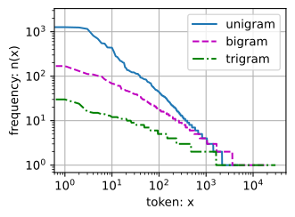
The tail is where count-based models die; generalizing models are the way forward.
Perplexity
Exponentiated average cross-entropy:
\operatorname{PPL} = \exp\left(-\frac{1}{T}\sum_{t=1}^{T} \log P(x_t \mid x_{<t})\right).
The effective branching factor: perfect prediction gives 1, a uniform guess gives |\mathcal{V}|.
def eval_nll(model, tokens):
    """Total negative log-likelihood of tokens, in nats."""
    return -sum(math.log(model.prob(tokens[:t], tokens[t]))
                for t in range(len(tokens)))

for n, model in models.items():
    ppl = math.exp(eval_nll(model, words_val) / len(words_val))
    print(f'{n}-gram held-out perplexity: {ppl:8.1f}')
1-gram held-out perplexity: 840.7
2-gram held-out perplexity: 775.1
3-gram held-out perplexity: 2618.1The trigram wrote the best text and scores the worst held-out perplexity: good samples and generalization are different things.
Bits per byte
Per-token metrics depend on what a token is. Divide total surprisal by bytes of text instead:
bpe = d2l.BPETokenizer(vocab_size=1024, pattern=d2l.BPETokenizer.GPT2_PATTERN)
bpe.train(text[:split])
streams = {'character': (list(text[:split]), list(text[split:]),
                         len(set(text))),
           'BPE (1,024)': (bpe.encode(text[:split]), bpe.encode(text[split:]),
                           bpe.vocab_size),
           'word': (words_train, words_val, vocab_size)}
n_bytes = len(text[split:].encode('utf-8'))
print(f'{"tokenization":>12} {"|V|":>5} {"tokens":>7} {"ppl":>8} {"bpb":>5}')
for name, (train, val, m) in streams.items():
    nll = eval_nll(NGramLM(train, 3, m), val)
    print(f'{name:>12} {m:>5} {len(val):>7} '
          f'{math.exp(nll / len(val)):>8.1f} {nll / math.log(2) / n_bytes:>5.2f}')
tokenization |V| tokens ppl bpb
character 27 17345 6.4 2.68
BPE (1,024) 1024 5509 281.6 2.58
word 4579 3373 2618.1 2.21Perplexity spans two orders of magnitude; bits per byte is nearly flat, and the ordering reverses. bpb is how modern LM training runs are compared across tokenizers.
Partitioning sequences
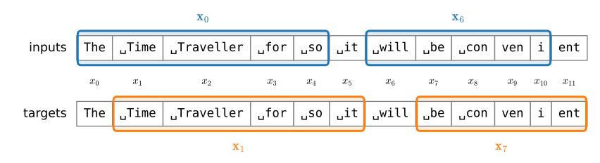
Overlapping length-5 windows of BPE token ids; targets are inputs shifted by one.
The data pipeline emits BPE ids
Train the 9.2 tokenizer, encode the corpus, lay out all overlapping windows (tokenization='char' recovers the character pipeline):
@d2l.add_to_class(d2l.TimeMachine)
def __init__(self, batch_size, num_steps, num_train=10000, num_val=5000,
             tokenization='bpe', vocab_size=1024):
    super(d2l.TimeMachine, self).__init__()
    self.save_hyperparameters()
    raw_text = self._download()
    if tokenization == 'bpe':
        self.tokenizer = d2l.BPETokenizer(
            vocab_size, pattern=d2l.BPETokenizer.GPT2_PATTERN)
        self.tokenizer.train(raw_text)
        corpus, self.vocab = self.tokenizer.encode(raw_text), self.tokenizer
    else:  # 'char': the character-level pipeline
        corpus, self.vocab = self.build(raw_text)
    array = d2l.tensor([corpus[i:i+num_steps+1]
                        for i in range(len(corpus)-num_steps)])
    self.X, self.Y = array[:,:-1], array[:,1:]
A minibatch: Y is X shifted by one token, and the ids decode back to Wells:
X: tf.Tensor(
[[109 754 275 285 298 104 277 286 682  44]
 [273 708 650 430 565 776 622 285 256 736]], shape=(2, 10), dtype=int32)
Y: tf.Tensor(
[[754 275 285 298 104 277 286 682  44 277]
 [708 650 430 565 776 622 285 256 736 316]], shape=(2, 10), dtype=int32)
X[0]: 'm going to wash and dress,'
Y[0]: ' going to wash and dress, and'
Recap
- Chain rule: language modeling is next-token prediction; generation, scoring, and prompted tasks all follow.
- n-grams: counts + smoothing; Zipf’s law makes the tables go sparse exponentially fast, so they memorize instead of generalize.
- Perplexity = effective branching factor, per token; bits per byte compares models across tokenizers.
- Training data: one stream of BPE ids, all overlapping windows, targets shifted by one. Every LM in the book trains on this.