Backpropagation Through Time

Backpropagation through time

Training an RNN is backpropagation on the unrolled graph: expand the recurrence one step at a time into a feedforward net where the same weights reappear at every step, then apply the chain rule and sum each weight’s gradient over all its occurrences (weight tying, as in a CNN).

The catch is length: a thousand-token sequence means a thousand matrix products forward, and another thousand back.

The gradient of a recurrence

Forward: h_t = f(x_t, h_{t-1}, w_\textrm{h}), o_t = g(h_t, w_\textrm{o}).

The hard factor is \partial h_t/\partial w_\textrm{h}: the weight acts at step t and through h_{t-1}. Writing f_t = f(x_t, h_{t-1}, w_\textrm{h}) and unrolling gives a sum over earlier steps, each a product of Jacobians:

\frac{\partial h_t}{\partial w_\textrm{h}} = \frac{\partial f_t}{\partial w_\textrm{h}} + \sum_{i=1}^{t-1}\Big(\prod_{j=i+1}^{t}\frac{\partial f_j}{\partial h_{j-1}}\Big) \frac{\partial f_i}{\partial w_\textrm{h}}.

Vanishing and exploding gradients

Make it linear: \mathbf{h}_t = \mathbf{W}_\textrm{hx}\mathbf{x}_t + \mathbf{W}_\textrm{hh}\mathbf{h}_{t-1}. Every Jacobian is the same matrix, so reaching back k steps multiplies by (\mathbf{W}_\textrm{hh}^\top)^{k}.

A matrix power is ruled by its eigenvalues (spectral radius \rho):

  • |\lambda| < 1: the term vanishes (\sim\rho^k \to 0).
  • |\lambda| > 1: the term explodes (\sim\rho^k \to \infty).
  • \rho = 1: the knife-edge.

Watch it happen

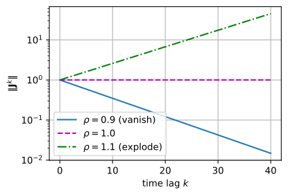
Operator norm \|\mathbf{J}^k\| of the k-step Jacobian product for a symmetric recurrence rescaled to spectral radius \rho (log scale):
np.random.seed(1)
h = 100
M = np.random.randn(h, h)
W = M + M.T                                # a random *symmetric* recurrence

def spectral_radius(A):
    return np.abs(np.linalg.eigvals(A)).max()

lags, norms = np.arange(41), []
for rho in (0.9, 1.0, 1.1):
    J = W * (rho / spectral_radius(W))     # rescale so that rho(J) = rho
    power, seq = np.eye(h), []
    for k in lags:
        seq.append(np.linalg.norm(power, 2))   # operator norm of J^k
        power = power @ J
    norms.append(seq)
    print(f'rho={rho}: ||J^40|| = {seq[-1]:.3g}')

d2l.plot(lags, norms, xlabel='time lag $k$', ylabel=r'$\|\mathbf{J}^k\|$',
         legend=[r'$\rho=0.9$ (vanish)', r'$\rho=1.0$', r'$\rho=1.1$ (explode)'],
         yscale='log', figsize=(4.5, 3))

rho=0.9: ||J^40|| = 0.0148
rho=1.0: ||J^40|| = 1
rho=1.1: ||J^40|| = 45.3

Three straight lines: decay, flat, blow-up. Over 40 steps the signal is amplified more than fortyfold or crushed below two percent.

Fix: arithmetic vs. architecture

  • Explosion is easy: rescale it. Gradient clipping caps the gradient norm before each update.
  • Vanishing cannot be rescaled away (scaling up noise only gives bigger noise). It needs a change of dynamics:
    • Gating (LSTM/GRU): a near-identity memory path, Jacobian \approx 1.
    • Linear recurrence / SSM: eigenvalues pinned inside the unit circle by construction, so \rho \le 1 is guaranteed, not hoped for.

Truncated BPTT

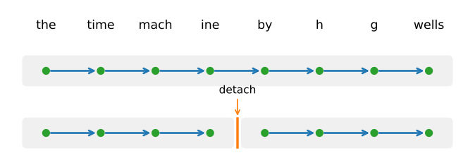
Full BPTT (top) vs. regular truncation into length-\tau segments (bottom), detaching the hidden state at each boundary.

Truncate the backward sum to \tau steps: the detach-state idiom. Cheaper and more stable; the bias (no dependency longer than \tau) is often a helpful regularizer.

Recap

  • BPTT = backprop on the unrolled recurrence; tied weights, summed gradients.
  • The k-step gradient carries a k-fold Jacobian product \sim\rho^k: vanish (\rho<1) or explode (\rho>1).
  • Clipping tames explosion; architecture (gates, stable linear recurrence) tames vanishing.
  • Truncation trades a little bias for stability and memory, the same store-vs.-recompute bargain as activation checkpointing at scale.