def f(x):
return 3 * x ** 2 - 4 * xCalculus
Dive into Deep Learning · §1.4
How a loss changes under a small parameter perturbation
limits · derivatives · gradients · the chain rule.
Derivatives indicate a direction of descent
Motivation
Training a model requires minimizing a loss. Calculus describes how that loss changes with the parameters:
- The derivative: how fast the loss moves when one parameter is perturbed.
- The gradient \nabla_\theta L: one slope per parameter, stacked.
- Optimizers step along -\nabla_\theta L: downhill.
- The chain rule differentiates nested functions.
01
Derivatives
limits, slopes, and where floating point gives out
It begins with a limit
Derivatives
Archimedes found a circle’s area with inscribed polygons. With n sides the polygon splits into n triangles whose areas sum to
n \cdot \tfrac{1}{2}\bigl(\tfrac{2\pi r}{n}\bigr)\, r = \pi r^2.
Taking n \to \infty is a limit, the idea at the root of all calculus.
As h → 0, the secant pivots into the tangent
Derivatives
The derivative of f at x is the limit of the difference quotient:
f'(x) = \lim_{h \to 0} \frac{f(x+h) - f(x)}{h}.
\tfrac{f(x+h)-f(x)}{h} is the slope of the secant through two points; as h \to 0 it pivots into the tangent, whose slope is f'(x).
One function by hand: f′(1) = 2
Derivatives
Let u = f(x) = 3x^2 - 4x. The rules (two slides ahead) give f'(x) = 6x - 4, so f'(1) = 2, the number the next two experiments must reproduce:
The quotient approaches 2, one digit per decade
Derivatives
At x = 1, shrinking h tenfold per row makes the difference quotient approach f'(1) = 2:
h=0.10000, numerical limit=2.30000
h=0.01000, numerical limit=2.03000
h=0.00100, numerical limit=2.00300
h=0.00010, numerical limit=2.00030
h=0.00001, numerical limit=2.00003
Successive rows give 2.3, 2.03, 2.003, …
Push h too far and the approximation fails
Derivatives · a warning
Smaller is not always better: f(1+h) and f(1) become nearly equal floats, and their difference loses its leading digits to cancellation:
h=1e-06, numerical limit=2.00000
h=1e-07, numerical limit=2.00000
h=1e-08, numerical limit=2.00000
h=1e-09, numerical limit=2.00000
h=1e-10, numerical limit=2.00000
h=1e-11, numerical limit=2.00000
h=1e-12, numerical limit=2.00018
h=1e-13, numerical limit=1.99840
h=1e-14, numerical limit=1.99840
h=1e-15, numerical limit=2.22045
h=1e-16, numerical limit=0.00000
Error creeps back in at h=10^{-12}; at 10^{-16}, when 1+h rounds to exactly 1, the quotient collapses to 0. This is a key reason autograd (the automatic-differentiation section) applies differentiation rules to recorded operations.
The picture: tangent of slope 2 at x = 1
Derivatives
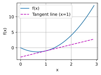
Plotting u = f(x) with the line y = 2x - 3 makes the number geometric: the tangent touches at (1, -1) and its slope is f'(1) = 2.
The d2l package wraps a few matplotlib helpers (set_figsize, plot, set_axes) reused throughout the book.
A handful of rules replaces the limit
Derivatives
Common derivatives
\dfrac{d}{dx} C = 0, \quad \dfrac{d}{dx} x^n = n\,x^{n-1},
\dfrac{d}{dx} e^x = e^x, \quad \dfrac{d}{dx}\ln x = \dfrac{1}{x}.
Combining functions
Sum: (f+g)' = f' + g'
Product: (fg)' = f g' + g f'
Quotient: \left(\dfrac{f}{g}\right)' = \dfrac{g f' - f g'}{g^2}
Apply them to 3x^2 - 4x: the derivative is 6x - 4, exactly what the limit experiment measured.
02
Partial derivatives & gradients
many inputs, one slope each
A partial derivative slices the surface
Gradients
For y = f(x_1, \ldots, x_n), the partial derivative \dfrac{\partial y}{\partial x_i} freezes every other variable and differentiates along one axis:
\frac{\partial y}{\partial x_i} = \lim_{h \to 0} \frac{f(\ldots, x_i + h, \ldots) - f(\ldots, x_i, \ldots)}{h}.
It is the slope of a 1-D slice through the surface.
The gradient points in the direction of steepest ascent
Gradients
Stack all n partials into the gradient \nabla f = [\partial_{x_1} f, \ldots, \partial_{x_n} f]^\top.
Along a unit direction \mathbf{u}, the rate of change is the dot product \nabla f^\top \mathbf{u}; by the linear-algebra section’s cosine formula this is largest when \mathbf{u} aligns with \nabla f. So the gradient is the direction of steepest ascent (proof via Cauchy–Schwarz, the multivariable-calculus section).
-\nabla f points downhill, which gives the gradient-descent direction.
Gradient identities: calculus done by linear algebra
Gradients
A few vector rules recur constantly; each is a linear-algebra-section operation (\nabla_{\mathbf{x}}\,\mathbf{A}\mathbf{x} = \mathbf{A}^\top is the transpose of the Jacobian; derivations in the matrix-calculus-and- automatic-differentiation section):
\nabla_{\mathbf{x}}\, \mathbf{A}\mathbf{x} = \mathbf{A}^\top
\nabla_{\mathbf{x}}\, \mathbf{x}^\top\mathbf{A} = \mathbf{A}
\nabla_{\mathbf{x}}\, \mathbf{x}^\top\mathbf{A}\mathbf{x} = (\mathbf{A} + \mathbf{A}^\top)\,\mathbf{x}
\nabla_{\mathbf{x}}\, \|\mathbf{x}\|^2 = 2\mathbf{x}
\nabla_{\mathbf{X}}\, \|\mathbf{X}\|_\textrm{F}^2 = 2\mathbf{X}
03
The chain rule
differentiating compositions, and a first look at backprop
The chain rule multiplies along the path
Chain rule
Deep networks are functions of functions of functions. For y = f(g(x)) with u = g(x):
\frac{dy}{dx} = \frac{dy}{du}\,\frac{du}{dx}.
Evaluate forward (x \to u \to y); accumulate derivatives backward.
The multivariate chain rule is a matrix–vector product
Chain rule
With m intermediates u_j, each depending on n inputs x_i, the sums \partial y/\partial x_i = \sum_j A_{ij}\, \partial y/\partial u_j assemble into
\nabla_{\mathbf{x}} y = \mathbf{A}\, \nabla_{\mathbf{u}} y, \qquad A_{ij} = \frac{\partial u_j}{\partial x_i}\ \text{(the transpose of the Jacobian, matrix-calculus section).}
A network’s gradient is a chain of such products: traversed forward it evaluates the function, traversed backward it computes every gradient. That backward pass is backpropagation (the backpropagation section).
This is why linear algebra is a prerequisite for deep learning.
Recap
Wrap-up
- Derivative = limit of the difference quotient = tangent slope; the numerical estimate improves as h shrinks, until cancellation takes over.
- Partials slice; the gradient stacks them and points uphill (-\nabla f downhill).
- Identities: \nabla \mathbf{A}\mathbf{x} = \mathbf{A}^\top, \nabla \|\mathbf{x}\|^2 = 2\mathbf{x}, …, all plain linear algebra.
- The chain rule multiplies along the path; multivariate, it is a matrix–vector product used in backpropagation.
- Next: autograd (the automatic-differentiation section) runs all of this by applying differentiation rules automatically.
Most optimization steps in this book use a gradient.