%matplotlib inline
from d2l import tensorflow as d2l
import numpy as np
from mpl_toolkits import mplot3d
import tensorflow as tfEmpirical risk vs. risk
Setup the modules and define a smooth risk f and a noisier empirical risk g (training loss):
def f(x):
    return x * d2l.cos(np.pi * x)

def g(x):
    return f(x) + 0.2 * d2l.cos(5 * np.pi * x)
The minimum of empirical risk on the training set is at a different location from the minimum of the population risk. Optimizing one doesn’t optimize the other:
def annotate(text, xy, xytext):
    d2l.plt.gca().annotate(text, xy=xy, xytext=xytext,
                           arrowprops=dict(arrowstyle='->'))

x = d2l.arange(0.5, 1.5, 0.01)
d2l.set_figsize((4.5, 2.5))
d2l.plot(x, [f(x), g(x)], 'x', 'risk')
annotate('min of\nempirical risk', (1.0, -1.2), (0.5, -1.1))
annotate('min of risk', (1.1, -1.05), (0.95, -0.5))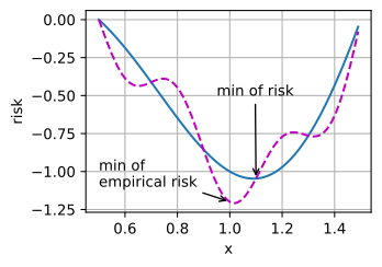
Local minima
f(x) = x \cos(\pi x) has multiple basins. Gradient descent stalls at the first one it falls into; only noise (e.g., SGD minibatch variance) can knock it out:
x = d2l.arange(-1.0, 2.0, 0.01)
d2l.plot(x, [f(x), ], 'x', 'f(x)')
annotate('local minimum', (-0.3, -0.25), (-0.77, -1.0))
annotate('global minimum', (1.1, -0.95), (0.6, 0.8))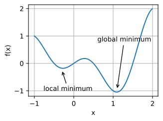
Saddle points
1D — f(x) = x^3 has f'(0) = 0 but it’s not a min:
x = d2l.arange(-2.0, 2.0, 0.01)
d2l.plot(x, [x**3], 'x', 'f(x)')
annotate('saddle point', (0, -0.2), (-0.52, -5.0))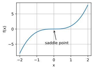
In high dim, with a Hessian of mixed signs, you get the classic saddle shape. Most zero-gradient points in deep learning are saddles, not minima — random Hessian eigenvalues are unlikely to all share a sign:
x, y = d2l.meshgrid(
    d2l.linspace(-1.0, 1.0, 101), d2l.linspace(-1.0, 1.0, 101))
z = x**2 - y**2

ax = d2l.plt.figure().add_subplot(111, projection='3d')
ax.plot_wireframe(x, y, z, **{'rstride': 10, 'cstride': 10})
ax.plot([0], [0], [0], 'rx')
ticks = [-1, 0, 1]
d2l.plt.xticks(ticks)
d2l.plt.yticks(ticks)
ax.set_zticks(ticks)
d2l.plt.xlabel('x')
d2l.plt.ylabel('y');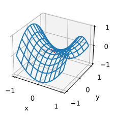
Vanishing gradients
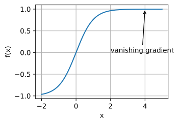
f(x) = \tanh(x) at x = 4: f'(4) \approx 0.0013. Gradient descent makes essentially no progress here. ReLU fixed this for activation functions; layer norm and residual connections fix it across deep networks.
x = d2l.arange(-2.0, 5.0, 0.01)
d2l.plot(x, [d2l.tanh(x)], 'x', 'f(x)')
annotate('vanishing gradient', (4, 1), (2, 0.0))