Minibatch Stochastic Gradient Descent

Minibatch SGD

GD: \mathcal{O}(n) per step, optimal use of data. SGD: \mathcal{O}(1) per step, noisy and one-at-a-time.

The compromise everyone uses: minibatch SGD — sample a batch of b examples, average their gradients:

\mathbf{x} \leftarrow \mathbf{x} - \frac{\eta}{b} \sum_{i \in \mathcal{B}} \nabla f_i(\mathbf{x}).

Why minibatches win

• Variance reduction — averaging b noisy gradients cuts variance by b.
• Hardware efficiency — GPUs do a batched matmul b\times faster than a loop over b single examples.

Vectorization and cache reuse are the real reason for batching, not just statistics.

Setup

%matplotlib inline
from d2l import tensorflow as d2l
import numpy as np
import tensorflow as tf
import time

A = tf.Variable(d2l.zeros((256, 256)))
B = tf.Variable(d2l.normal([256, 256], 0, 1))
C = tf.Variable(d2l.normal([256, 256], 0, 1))

class Timer:
    """Record multiple running times."""
    def __init__(self):
        self.times = []
        self.start()

    def start(self):
        """Start the timer."""
        self.tik = time.time()

    def stop(self):
        """Stop the timer and record the time in a list."""
        self.times.append(time.time() - self.tik)
        return self.times[-1]

    def avg(self):
        """Return the average time."""
        return sum(self.times) / len(self.times)

    def sum(self):
        """Return the sum of time."""
        return sum(self.times)

    def cumsum(self):
        """Return the accumulated time."""
        return np.array(self.times).cumsum().tolist()

timer = Timer()

Three loops, three speeds

Compute \mathbf{A} = \mathbf{B}\mathbf{C} on 256 \times 256 matrices in three increasingly vectorized ways:

# Compute A = BC one element at a time
timer.start()
for i in range(256):
    for j in range(256):
        A[i, j].assign(tf.tensordot(B[i, :], C[:, j], axes=1))
timer.stop()

99.45890092849731

timer.start()
for j in range(256):
    A[:, j].assign(tf.tensordot(B, C[:, j], axes=1))
timer.stop()

0.2929561138153076

timer.start()
A.assign(tf.tensordot(B, C, axes=1))
timer.stop()

gigaflops = [0.03 / i for i in timer.times]
print(f'performance in Gigaflops: element {gigaflops[0]:.3f}, '
      f'column {gigaflops[1]:.3f}, full {gigaflops[2]:.3f}')

performance in Gigaflops: element 0.000, column 0.102, full 11.222

Element-wise → column-wise → matrix-wise: typically two orders of magnitude difference. The cache and SIMD do the work; the loop is overhead.

The minibatch sweet spot

• b = 1: high gradient variance, GPU mostly idle.
• b = n: full GD — best variance, slowest progress.
• b = 32 \ldots 1024: enough work to fill the GPU, variance reduced by \sqrt{b}.

In practice, batch size is constrained more by memory and parallelism than by statistics. Modern training: 256 to 65k+ on accelerators.

timer.start()
for j in range(0, 256, 64):
    A[:, j:j+64].assign(tf.tensordot(B, C[:, j:j+64], axes=1))
timer.stop()
print(f'performance in Gigaflops: block {0.03 / timer.times[3]:.3f}')

performance in Gigaflops: block 1.551

Airfoil dataset

Real regression dataset for the experiments — 1503 examples, 5 features, 1 target:

d2l.DATA_HUB['airfoil'] = (d2l.DATA_URL + 'airfoil_self_noise.dat',
                           '76e5be1548fd8222e5074cf0faae75edff8cf93f')


def get_data_ch11(batch_size=10, n=1500):
    data = np.genfromtxt(d2l.download('airfoil'),
                         dtype=np.float32, delimiter='\t')
    data = (data - data.mean(axis=0)) / data.std(axis=0)
    data_iter = d2l.load_array((data[:n, :-1], data[:n, -1]),
                               batch_size, is_train=True)
    return data_iter, data.shape[1]-1

Manual SGD update

First isolate the optimizer step. For minibatch size b, average the gradients and move each parameter by -\eta \nabla f_{\mathcal{B}}:

def sgd(params, grads, states, hyperparams):
    for param, grad in zip(params, grads):
        param.assign_sub(hyperparams['lr']*grad)

Generic training loop

The reusable trainer initializes a tiny linear model, runs forward/backward on each minibatch, and records loss against wall-clock time:

def train_ch11(trainer_fn, states, hyperparams, data_iter,
               feature_dim, num_epochs=2):
    # Initialization
    w = tf.Variable(tf.random.normal(shape=(feature_dim, 1),
                                   mean=0, stddev=0.01),trainable=True)
    b = tf.Variable(tf.zeros(1), trainable=True)

    # Train
    net, loss = lambda X: d2l.linreg(X, w, b), d2l.squared_loss
    animator = d2l.Animator(xlabel='epoch', ylabel='loss',
                            xlim=[0, num_epochs], ylim=[0.22, 0.35])
    n, timer = 0, d2l.Timer()

    for _ in range(num_epochs):
        for X, y in data_iter:
          with tf.GradientTape() as g:
            l = tf.math.reduce_mean(loss(net(X), y))

          dw, db = g.gradient(l, [w, b])
          trainer_fn([w, b], [dw, db], states, hyperparams)
          n += X.shape[0]
          if n % 200 == 0:
              timer.stop()
              p = n/X.shape[0]
              q = p/tf.data.experimental.cardinality(data_iter).numpy()
              r = (d2l.evaluate_loss(net, data_iter, loss),)
              animator.add(q, r)
              timer.start()
    print(f'loss: {animator.Y[0][-1]:.3f}, {timer.sum()/num_epochs:.3f} sec/epoch')
    return timer.cumsum(), animator.Y[0]

Full-batch baseline

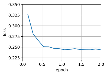
Set b to the whole dataset. Each epoch gives only one update, so the curve is smooth but progress per second is poor:

def train_sgd(lr, batch_size, num_epochs=2):
    data_iter, feature_dim = get_data_ch11(batch_size)
    return train_ch11(
        sgd, None, {'lr': lr}, data_iter, feature_dim, num_epochs)

gd_res = train_sgd(1, 1500, 10)

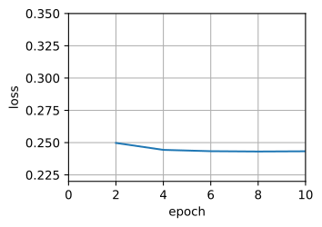
loss: 0.243, 0.088 sec/epoch

Comparing batch sizes

b = 1500 (full batch), b = 1 (pure SGD), b = 100, b = 10 — same model, same total epochs:

sgd_res = train_sgd(0.005, 1)

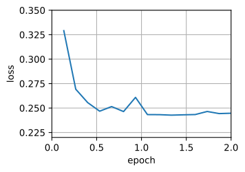
loss: 0.245, 4.737 sec/epoch

mini1_res = train_sgd(.4, 100)

loss: 0.245, 0.071 sec/epoch

Pure SGD updates often but wastes vector hardware. b=100 processes enough examples per step to make each update cheap and stable.

Wall-clock view

mini2_res = train_sgd(.05, 10)

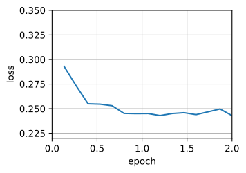
loss: 0.243, 0.499 sec/epoch

d2l.set_figsize([6, 3])
d2l.plot(*list(map(list, zip(gd_res, sgd_res, mini1_res, mini2_res))),
         'time (sec)', 'loss', xlim=[1e-2, 10],
         legend=['gd', 'sgd', 'batch size=100', 'batch size=10'])
d2l.plt.gca().set_xscale('log')

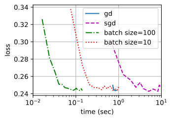
Read the x-axis as elapsed time, not examples processed: minibatches win because they make each second of compute do more useful linear algebra.

Concise: framework optimizer

Same experiment using the framework’s built-in SGD optimizer — fewer lines, same numbers:

def train_concise_ch11(trainer_fn, hyperparams, data_iter, num_epochs=2):
    # Initialization
    net = tf.keras.Sequential()
    net.add(tf.keras.layers.Dense(1,
            kernel_initializer=tf.random_normal_initializer(stddev=0.01)))
    optimizer = trainer_fn(**hyperparams)
    loss = tf.keras.losses.MeanSquaredError()
    animator = d2l.Animator(xlabel='epoch', ylabel='loss',
                            xlim=[0, num_epochs], ylim=[0.22, 0.35])
    n, timer = 0, d2l.Timer()
    for _ in range(num_epochs):
        for X, y in data_iter:
            with tf.GradientTape() as g:
                out = net(X)
                l = loss(y, out)
                params = net.trainable_variables
                grads = g.gradient(l, params)
            optimizer.apply_gradients(zip(grads, params))
            n += X.shape[0]
            if n % 200 == 0:
                timer.stop()
                p = n/X.shape[0]
                q = p/tf.data.experimental.cardinality(data_iter).numpy()
                # `MeanSquaredError` computes squared error without the 1/2
                # factor
                r = (d2l.evaluate_loss(net, data_iter, loss) / 2,)
                animator.add(q, r)
                timer.start()
    print(f'loss: {animator.Y[0][-1]:.3f}, {timer.sum()/num_epochs:.3f} sec/epoch')

data_iter, _ = get_data_ch11(10)
trainer = tf.keras.optimizers.SGD
train_concise_ch11(trainer, {'learning_rate': 0.05}, data_iter)

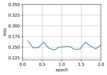
loss: 0.255, 0.934 sec/epoch

Recap

• Minibatch SGD interpolates between GD and pure SGD.
• Vectorization and cache reuse make b > 1 vastly cheaper per example — that’s why everyone uses minibatches even setting statistics aside.
• Variance scales as 1/b; convergence rate has a \sqrt{b} effective step size advantage over single-example.
• Choose b to fill the accelerator, not to optimize the bias/variance tradeoff theoretically.