Step 1: Attend

Natural Language Inference: Using Attention

Decomposable Attention

Decomposable Attention (Parikh et al., 2016) — a small, fast NLI model that beat much more complex recurrence-based architectures on SNLI in 2016. No recurrence, no convolution — pure attention + MLPs.

Three steps: Attend → Compare → Aggregate.

Pipeline

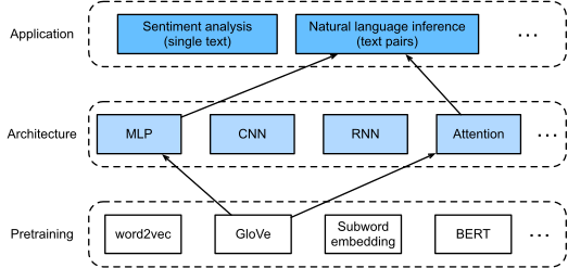
GloVe → attend → compare → aggregate → 3-way classifier.

The decomposable attention model

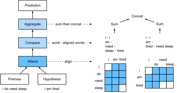
Align premise/hypothesis tokens, then compare and aggregate.

Setup

from d2l import tensorflow as d2l
import tensorflow as tf
import keras

Compute alignment weights between every premise word and every hypothesis word. Use them to build aligned context vectors:

def mlp(num_hiddens, flatten):
    net = keras.Sequential()
    net.add(keras.layers.Dropout(0.2))
    net.add(keras.layers.Dense(num_hiddens, activation='relu'))
    if flatten:
        net.add(keras.layers.Flatten())
    net.add(keras.layers.Dropout(0.2))
    net.add(keras.layers.Dense(num_hiddens, activation='relu'))
    if flatten:
        net.add(keras.layers.Flatten())
    return net

class Attend(keras.layers.Layer):
    def __init__(self, num_hiddens, **kwargs):
        super(Attend, self).__init__(**kwargs)
        self.f = mlp(num_hiddens=num_hiddens, flatten=False)

    def call(self, A, B):
        # Shape of `A`/`B`: (`batch_size`, no. of tokens in sequence A/B,
        # `embed_size`)
        # Shape of `f_A`/`f_B`: (`batch_size`, no. of tokens in sequence A/B,
        # `num_hiddens`)
        f_A = self.f(A)
        f_B = self.f(B)
        # Shape of `e`: (`batch_size`, no. of tokens in sequence A,
        # no. of tokens in sequence B)
        e = tf.matmul(f_A, tf.transpose(f_B, perm=[0, 2, 1]))
        # Shape of `beta`: (`batch_size`, no. of tokens in sequence A,
        # `embed_size`), where sequence B is softly aligned with each token
        # (axis 1 of `beta`) in sequence A
        beta = tf.matmul(tf.nn.softmax(e, axis=-1), B)
        # Shape of `alpha`: (`batch_size`, no. of tokens in sequence B,
        # `embed_size`), where sequence A is softly aligned with each token
        # (axis 1 of `alpha`) in sequence B
        alpha = tf.matmul(
            tf.nn.softmax(tf.transpose(e, perm=[0, 2, 1]), axis=-1), A)
        return beta, alpha

Step 2: Compare

For each premise word a_i, run an MLP on [a_i, \beta_i] where \beta_i is the soft-aligned hypothesis context. Same for hypothesis words:

class Compare(keras.layers.Layer):
    def __init__(self, num_hiddens, **kwargs):
        super(Compare, self).__init__(**kwargs)
        self.g = mlp(num_hiddens=num_hiddens, flatten=False)

    def call(self, A, B, beta, alpha):
        V_A = self.g(tf.concat([A, beta], axis=2))
        V_B = self.g(tf.concat([B, alpha], axis=2))
        return V_A, V_B

Step 3: Aggregate

Sum the per-token compared vectors → concat the two sentence summaries → final MLP → 3-way logits:

class Aggregate(keras.layers.Layer):
    def __init__(self, num_hiddens, num_outputs, **kwargs):
        super(Aggregate, self).__init__(**kwargs)
        self.h = mlp(num_hiddens=num_hiddens, flatten=True)
        self.linear = keras.layers.Dense(num_outputs)

    def call(self, V_A, V_B):
        # Sum up both sets of comparison vectors
        V_A = tf.reduce_sum(V_A, axis=1)
        V_B = tf.reduce_sum(V_B, axis=1)
        # Feed the concatenation of both summarization results into an MLP
        Y_hat = self.linear(self.h(tf.concat([V_A, V_B], axis=1)))
        return Y_hat

Putting it together

The final module wires the three stages into one classifier. Inputs are premise IDs and hypothesis IDs; output is 3 logits for entailment, contradiction, and neutral.

class DecomposableAttention(keras.Model):
    def __init__(self, vocab, embed_size, num_hiddens, **kwargs):
        super(DecomposableAttention, self).__init__(**kwargs)
        self.embedding = keras.layers.Embedding(len(vocab), embed_size)
        self.attend = Attend(num_hiddens)
        self.compare = Compare(num_hiddens)
        # There are 3 possible outputs: entailment, contradiction, and neutral
        self.aggregate = Aggregate(num_hiddens, 3)

    def call(self, inputs, training=False, **kwargs):
        premises, hypotheses = inputs
        A = self.embedding(premises)
        B = self.embedding(hypotheses)
        beta, alpha = self.attend(A, B)
        V_A, V_B = self.compare(A, B, beta, alpha)
        Y_hat = self.aggregate(V_A, V_B)
        return Y_hat

Loading data + model

SNLI examples are padded premise/hypothesis pairs. Initialize the model with GloVe embeddings, then train all MLP stages end-to-end:

batch_size, num_steps = 256, 50
train_iter, test_iter, vocab = d2l.load_data_snli(batch_size, num_steps)

read 549367 examples
read 9824 examples

embed_size, num_hiddens, devices = 100, 200, d2l.try_all_gpus()
net = DecomposableAttention(vocab, embed_size, num_hiddens)
glove_embedding = d2l.TokenEmbedding('glove.6b.100d')
embeds = glove_embedding[vocab.idx_to_token]
# Build the embedding layer before assigning pretrained weights.
net.embedding.build((None,))
net.embedding.set_weights([embeds])

Training

Loss should fall quickly: there is no recurrence, so every token-pair alignment and every MLP comparison is fully parallelizable.

lr, num_epochs = 0.001, 4
# Wrap tf.data batches: each yields (premises, hypotheses, labels);
# Keras model expects (X, y) where X = (premises, hypotheses)
def reformat(premises, hypotheses, labels):
    return (premises, hypotheses), labels

train_iter_tf = train_iter.map(reformat)
test_iter_tf = test_iter.map(reformat)
net.compile(optimizer=keras.optimizers.Adam(lr),
            loss=keras.losses.SparseCategoricalCrossentropy(from_logits=True),
            metrics=['accuracy'])
net.fit(train_iter_tf, validation_data=test_iter_tf, epochs=num_epochs)

Epoch 1/4
Final epoch metrics: accuracy: 0.3281 - loss: 4.0683
Final epoch metrics: accuracy: 0.3148 - loss: 4.3249
Final epoch metrics: accuracy: 0.3260 - loss: 3.4287
Final epoch metrics: accuracy: 0.3315 - loss: 2.9140
Final epoch metrics: accuracy: 0.3364 - loss: 2.6008
...
Final epoch metrics: accuracy: 0.7942 - loss: 0.5206
Final epoch metrics: accuracy: 0.7942 - loss: 0.5206
Final epoch metrics: accuracy: 0.7942 - loss: 0.5205
Final epoch metrics: accuracy: 0.7942 - loss: 0.5205

Final epoch metrics: accuracy: 0.7949 - loss: 0.5184 - val_accuracy: 0.8150 - val_loss: 0.4777

Predict

Read the examples semantically: “he is good” follows from “he is great”, while “he is bad” contradicts it. The model’s label mapping should reflect that ordering.

def predict_snli(net, vocab, premise, hypothesis):
    """Predict the logical relationship between the premise and hypothesis."""
    premise = tf.constant([vocab[premise]], dtype=tf.int32)
    hypothesis = tf.constant([vocab[hypothesis]], dtype=tf.int32)
    label = tf.argmax(net((premise, hypothesis), training=False), axis=1)
    return 'entailment' if label == 0 else 'contradiction' if label == 1 \
            else 'neutral'

predict_snli(net, vocab, ['he', 'is', 'good', '.'], ['he', 'is', 'bad', '.'])

'contradiction'

Recap

Decomposable Attention does NLI in three small MLP stages: attend, compare, aggregate.
No recurrence — completely parallelizable; trains fast even before GPU acceleration was abundant.
A precursor to the cross-attention machinery that BERT (next deck) does end-to-end inside one Transformer encoder.