The \tfrac{1}{2} is cosmetic: it cancels the 2 from differentiating the square.
\ell_2-regularized linear regression is the classic ridge regression; the \ell_1 version is lasso.
Ridge shrinks, lasso selects
The geometry
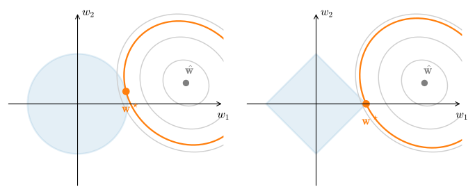
A budget \|\mathbf{w}\| \le t turns the penalty into a constraint: the answer is where a loss contour first touches the constraint region.
Loss contours centred on the unconstrained optimum \hat{\mathbf{w}} grow until they meet the constraint at \mathbf{w}^\star. Left (\ell_2 ball): contact is tangential, so both coordinates shrink. Right (\ell_1 diamond): contact is at a corner, forcing w_2 to exactly zero.
A round ball generally produces continuous shrinkage without exact zeros; a pointed diamond can touch at a corner, producing sparsity. Thus lasso can perform feature selection whereas ridge generally does not.
Why it is called weight decay
The update
The penalty adds \lambda\mathbf{w} to the gradient, so each SGD step gains a shrink factor:
Nothing else changes: same linear model, same squared loss. The loss includes the penalty scaled by lambd.
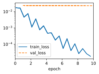
\lambda = 0: training and validation diverge
From Scratch · the overfit
train_scratch(0)
L2 norm of w: 0.011104541830718517
Training loss decreases sharply while validation loss remains high. The printed \|\mathbf{w}\|^2 shows that the unregularized fit uses large weights.
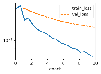
\lambda = 3: regularization reduces the gap
From Scratch · the rescue
train_scratch(3)
L2 norm of w: 0.0003025034093298018
Training loss is higher, but validation loss decreases and \|\mathbf{w}\|^2 is an order of magnitude smaller.
Why shrinkage helps: damp directions weakly constrained by the data
From Scratch · the why
Ridge keeps a closed form, and the SVD \mathbf{X} = \mathbf{U}\mathbf{D}\mathbf{V}^\top shows exactly what shrinks: the response along the j-th principal direction is damped by
Strong directions (d_j large) pass through nearly untouched; the weakly constrained ones are suppressed hardest.
Twenty examples pin down at most 20 of 200 directions (\textrm{df}(0) = 20); \lambda = 3 prices the model at \textrm{df} \approx 15 effective parameters.
02
Framework Implementations
where the framework keeps the decay
Decay as a layer regularizer
Concise · TensorFlow
Keras attaches the penalty to the layer via kernel_regularizer, then surfaces it through net.losses:
class WeightDecay(d2l.LinearRegression):def__init__(self, wd, lr):super().__init__(lr)self.save_hyperparameters()# Keras' l2(wd) penalty is wd*sum(w**2) (no 1/2 factor), so use# wd/2 to match the (wd/2)*||w||^2 convention used elsewhere.self.net = tf.keras.layers.Dense(1, kernel_regularizer=tf.keras.regularizers.l2(wd /2), kernel_initializer=tf.keras.initializers.RandomNormal(0, 0.01) )def loss(self, y_hat, y):returnsuper().loss(y_hat, y) + tf.add_n(self.net.losses)
Keras’ l2(wd) has no\tfrac{1}{2} factor, so we pass wd / 2 to match the convention used from scratch.
Same effect, less code
Concise · result
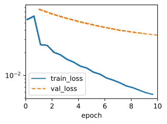
Fit with wd = 3: the validation curve matches the from-scratch run.
L2 norm of w: 0.00038615940138697624
A framework’s weight_decay adds \lambda\mathbf{w} to the gradient; the scratch penalty added \tfrac{\lambda}{2}\|\mathbf{w}\|^2 to the loss. Converged norms need not match exactly, only the effect.
The adaptive-optimizer reading: AdamW
Beyond linear models
Inside an Adam-style update each coordinate gets its own step size, so folding the penalty into the gradient rescales it per coordinate: it stops being uniform shrinkage.
Decoupling the decay from the adaptive step restores the intent of plain 1-\eta\lambda shrinkage. This is AdamW, a default for training large models.
For deep networks, weight decay is commonly applied to every layer’s weights, with exceptions such as biases configured separately.
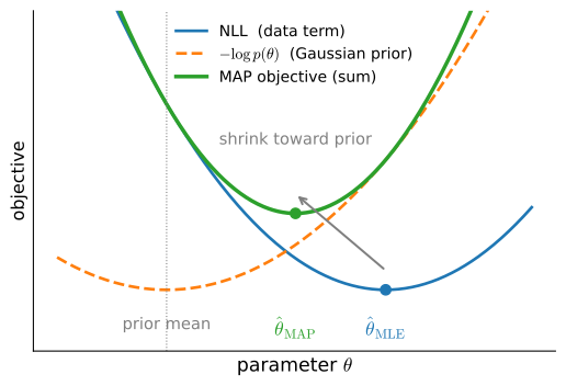
MAP = MLE + a prior. The linear-regression section obtained squared loss from Gaussian noise; a Gaussian prior on \mathbf{w} adds weight decay, with \lambda=\sigma^2/(n\tau^2) under the averaged-loss convention.
A Gaussian prior centred at zero pulls the maximum-likelihood estimate back toward the origin.
Summary
Wrap-up
Weight decay = original loss +\ \tfrac{\lambda}{2}\|\mathbf{w}\|_2^2; per step it shrinks the weights by 1 - \eta\lambda before the data update.
Spectral view: each direction damped by d_j^2/(d_j^2+\tilde\lambda); the 200-knob model ran at \textrm{df} \approx 15 effective parameters, a continuous dial tuned on a validation set.
The 20{\times}200 rig: \lambda=0 memorizes; \lambda=3 trades training error for a falling validation loss.
Frameworks expose decay in the optimizer (or layer / gradient transform).
Same idea scales up: AdamW for big models, a Gaussian prior in disguise.