Real images have channels: RGB has 3, while deep CNN feature maps may have hundreds or thousands.
Going deeper, networks often trade spatial resolution for channel depth, representing more feature types at fewer locations.
This deck:
Multiple input channels — kernels grow a 3rd axis.
Multiple output channels — stack many filters.
1 \times 1 convolutions — pure channel mixing.
Multi-input-channel convolution
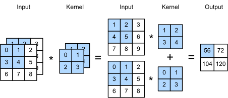
With c_i input channels, the kernel becomes c_i \times k_h \times k_w — a 2D filter per input channel. The output is the sum of per-channel cross-correlations:
from d2l import tensorflow as d2limport tensorflow as tf
def corr2d_multi_in(X, K):# Iterate through the 0th dimension (channel) of K first, then add them upreturn tf.reduce_sum([d2l.corr2d(x, k) for x, k inzip(X, K)], axis=0)
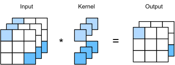
Each output channel comes from its own set of input-channel filters. Stack c_o such filter sets to get a 4-D kernel of shape c_o \times c_i \times k_h \times k_w:
Intuition: each of the c_o output channels is a different combination of inputs, learned to detect a different feature. Together, the channels form a learned feature representation.
Output channels in code
Apply the multi-input-channel function c_o times and stack the results along a new leading axis:
def corr2d_multi_in_out(X, K):# Iterate through the 0th dimension of K, and each time, perform# cross-correlation operations with input X. All of the results are# stacked togetherreturn d2l.stack([corr2d_multi_in(X, k) for k in K], 0)
Verify multi-output convolution
Build a 3-output-channel kernel by stacking three offset copies:
A conv layer with c_o outputs, c_i inputs, and a k_h \times k_w kernel has
c_o \cdot c_i \cdot k_h \cdot k_w \;+\; c_o
learnable parameters. Standard sizes:
3 → 64 channels, 3×3 kernel: 1.7k weights.
256 → 256 channels, 3×3 kernel: 590k weights.
512 → 2048 channels, 3×3 kernel: 9.4M weights.
If input and output channel counts grow together, parameter count grows quadratically, which constrains how quickly networks can widen.
The 1×1 convolution
A 1 \times 1 kernel has no spatial extent beyond its current position.
Because it acts as a per-pixel fully connected layer across channels. At every spatial position, it computes a linear combination of the c_i input channels into the c_o output channels:
1×1 conv: 3 input channels × 2 output channels. Each output pixel = a 2×3 matrix-vector product on the input channel vector at that position.
1×1 conv as matmul
At each pixel, the 1×1 conv applies the same c_o \times c_i matrix to the input channel vector. Reshape the spatial axes out and it’s a single matrix multiply:
def corr2d_multi_in_out_1x1(X, K): c_i, h, w = X.shape c_o = K.shape[0] X = d2l.reshape(X, (c_i, h * w)) K = d2l.reshape(K, (c_o, c_i))# Matrix multiplication in the fully connected layer Y = d2l.matmul(K, X)return d2l.reshape(Y, (c_o, h, w))
Bottlenecks (ResNet) — squeeze channels with 1×1, do expensive 3×3 in the smaller space, expand back with 1×1, reducing the cost of the spatial convolution. The exact saving depends on channel widths and can be \sim 4× overall.
Pointwise convs (MobileNet) — depthwise 3×3 + pointwise 1×1 splits a regular conv into two cheaper pieces.
Squeeze-and-Excitation, attention heads — wherever you need cheap channel mixing without changing resolution.
Grouped and depthwise convolutions
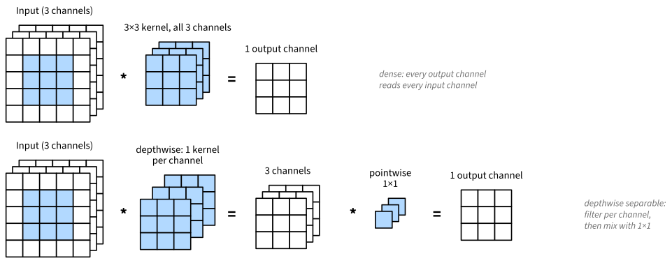
A dense conv connects every input channel to every output channel. Split the channels into g groups and convolve each group separately: parameters and compute drop by a factor of g (as in ResNeXt).
The extreme g = c_i = c_o is a depthwise convolution: one k \times k filter per channel, no channel mixing at all.
Dense conv mixes all input channels; depthwise filters each channel separately; pointwise 1×1 mixes them back.
Depthwise-separable convolutions
Factor spatial filtering from channel mixing: depthwise k \times k, then pointwise 1 \times 1 (MobileNet, Xception).
\frac{\text{separable cost}}{\text{dense cost}} = \frac{1}{c_o} + \frac{1}{k^2} \approx \frac{1}{9} \;\text{ for } k = 3.
A h \times w image with k \times k kernel and c_i \to c_o channels takes
\mathcal{O}(h \cdot w \cdot k^2 \cdot c_i \cdot c_o)
operations. For a 256×256 image, 5×5 kernel, and 128→128 channels, counting multiplications and additions separately gives more than 53 billion operations for one layer.
Consequently:
Convolutions benefit from GPU and TPU acceleration.
Efficient architectures use 1×1 bottlenecks, depthwise-separable convolutions, and grouped convolutions to reduce channel costs.
Recap
Multi-input-channel: per-channel kernel, results summed across input channels.
Multi-output-channel: stack independent filter banks; one output channel per filter set.
Total weights: c_o c_i k_h k_w + c_o.
1\times 1 convolutions are per-pixel fully connected layers across channels and are widely used in bottlenecks and pointwise convolutions.
Compute scales linearly with c_i \cdot c_o — the dominant cost in deep CNNs.