class DWSBlock(tf.keras.layers.Layer):
    """Depthwise 3x3 and pointwise 1x1 convolutions, each with BN and ReLU."""
    def __init__(self, out_channels, strides=1):
        super().__init__()
        self.net = tf.keras.models.Sequential([
            tf.keras.layers.DepthwiseConv2D(
                kernel_size=3, strides=strides, padding='same',
                use_bias=False, depthwise_initializer='he_normal'),
            tf.keras.layers.BatchNormalization(momentum=0.9),
            tf.keras.layers.ReLU(),
            tf.keras.layers.Conv2D(out_channels, kernel_size=1,
                                   use_bias=False,
                                   kernel_initializer='he_normal'),
            tf.keras.layers.BatchNormalization(momentum=0.9),
            tf.keras.layers.ReLU()])

    def call(self, X):
return self.net(X)Efficient ConvNets: Depthwise Separability, Mobile Architectures, and Re-parameterization
Where convnets still win
Most deployed convnets run on phones, cameras, cars, and embedded boards: budgets in milliseconds and milliwatts. Three ideas organize the efficient regime:
- Factorize: depthwise-separable convolutions (MobileNet).
- Scale and search: let optimization allocate width, depth, resolution (EfficientNet, MobileNetV4).
- Re-parameterize: train a multi-branch net, ship an algebraically identical single-branch one (RepVGG).
Depthwise separability, recalled
A dense k \times k convolution factorizes into a per-channel spatial filter plus a 1 \times 1 channel mixture, at fraction
\frac{1}{c_\textrm{o}} + \frac{1}{k^2}
of the dense cost: roughly 1/9 for 3 \times 3 kernels.
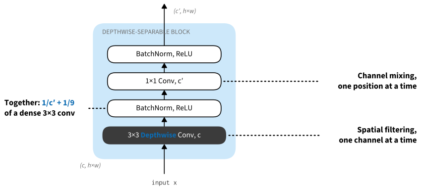
The depthwise stage filters each channel; the pointwise stage mixes channels; BN and ReLU follow each.
The block in code
MobileNet is this block, stacked; stride-2 depthwise convolutions downsample, so there is no pooling:
Mini-MobileNet
Like VGG, the network is a list of block parameters, here (channels, stride) pairs:
class MiniMobileNet(d2l.Classifier):
    def __init__(self, arch=((64, 1), (128, 2), (128, 1), (256, 2), (256, 1),
                             (512, 2), (512, 1)),
                 lr=0.1, num_classes=10):
        super().__init__()
        self.save_hyperparameters()
        self.net = tf.keras.models.Sequential([
            tf.keras.layers.Conv2D(32, kernel_size=3, strides=2,
                                   padding='same', use_bias=False,
                                   kernel_initializer='he_normal'),
            tf.keras.layers.BatchNormalization(momentum=0.9),
            tf.keras.layers.ReLU()])
        for out_channels, strides in arch:
            self.net.add(DWSBlock(out_channels, strides))
        self.net.add(tf.keras.layers.GlobalAvgPool2D())
        self.net.add(tf.keras.layers.Dense(num_classes))

    def configure_optimizers(self):
return tf.keras.optimizers.SGD(self.lr, momentum=0.9)Matched parameter budget
Same parameter budget, same head, 10 epochs of Fashion-MNIST at 96×96; the dense net must stop at 128 channels where the separable one reaches 512:
mini-MobileNet: 542,474 params, val acc 0.913
VGG-style: 583,594 params, val acc 0.922
Accuracy is comparable across frameworks and seeds; the ordering of the two models is noise. Mini-MobileNet uses 7.7\times fewer multiply-adds (50M vs. 385M), but its epochs are only about 2–3\times faster: FLOPs are not latency (depthwise convolutions are memory-bound).
The inverted bottleneck
ResNet bottlenecks compress around the expensive dense 3×3. Once the 3×3 is depthwise, wide is cheap and MobileNetV2 inverts the block:
- thin residual stream, 1 \times 1 expansion (6×),
- depthwise 3×3 in the wide space,
- linear 1 \times 1 projection back (no ReLU: it would destroy information in the thin space).
The tensors retained across blocks are the narrow ones, so activation memory stays small. ConvNeXt reused this exact shape with a 7×7 depthwise convolution.
Scaling and searching
- EfficientNet: scale depth, width, resolution together (\alpha^\phi, \beta^\phi, \gamma^\phi, one budget knob \phi); base block found by architecture search.
- EfficientNetV2: search rewards training speed; drops depthwise blocks from early high-resolution stages (memory-bound there) and grows image size during training.
- MobileNetV4: one universal inverted bottleneck covering four block variants; searched to be near Pareto-optimal across phone CPUs, DSPs, GPUs, and NPUs.
The block is human insight; the allocation is an optimization problem against measured latency.
RepVGG: train branches, ship a stack
Multi-branch nets train better (ResNet’s lesson); plain 3×3 stacks run faster (one big kernel per layer, one live tensor). RepVGG gets both: train with branches, then fuse them exactly.
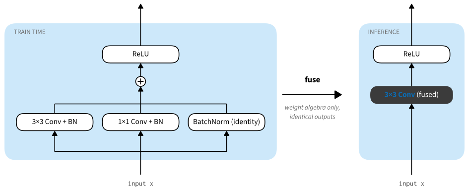
Train-time: 3×3 + 1×1 + identity, each with BN. Inference: one 3×3 convolution, same function.
The train-time block
class RepVGGBlock(tf.keras.Model):
    """Train-time block: 3x3, 1x1, and identity branches, each with BN."""
    def __init__(self, num_channels):
        super().__init__()
        self.conv3 = tf.keras.layers.Conv2D(num_channels, 3, padding='same',
                                            use_bias=False)
        self.conv1 = tf.keras.layers.Conv2D(num_channels, 1, use_bias=False)
        self.bn3 = tf.keras.layers.BatchNormalization(epsilon=1e-5)
        self.bn1 = tf.keras.layers.BatchNormalization(epsilon=1e-5)
        self.bn0 = tf.keras.layers.BatchNormalization(epsilon=1e-5)

    def call(self, X, training=False):
        return tf.keras.activations.relu(
            self.bn3(self.conv3(X), training=training)
            + self.bn1(self.conv1(X), training=training)
            + self.bn0(X, training=training))
The fusion algebra
Three pieces of weight algebra, all exact:
- Fold BN into the conv (per output channel o):
\hat{\mathbf{W}}_o = \frac{\gamma_o}{\sqrt{\sigma_o^2+\epsilon}}\,\mathbf{W}_o, \qquad \hat{b}_o = \beta_o - \frac{\gamma_o \mu_o}{\sqrt{\sigma_o^2+\epsilon}}.
- A 1 \times 1 kernel is a 3 \times 3 kernel padded with zeros; the identity is a 3 \times 3 kernel with a centered 1 where i = o.
- Convolution is linear in its kernel: sum the three kernels and the three biases.
Fusing in code
def fuse_bn(W, bn):
    scale = bn.gamma / tf.sqrt(bn.moving_variance + bn.epsilon)
    return W * scale, bn.beta - bn.moving_mean * scale

def fuse_block(blk):
    c = blk.conv3.kernel.shape[-1]
    pad = [[1, 1], [1, 1], [0, 0], [0, 0]]
    W3, b3 = fuse_bn(blk.conv3.kernel, blk.bn3)
    W1, b1 = fuse_bn(tf.pad(blk.conv1.kernel, pad), blk.bn1)
    I = tf.pad(tf.reshape(tf.eye(c), (1, 1, c, c)), pad)
    W0, b0 = fuse_bn(I, blk.bn0)
    return W3 + W1 + W0, b3 + b1 + b0
Exact to the last float
Push a few batches through to populate the BN running statistics, then compare the three-branch block against the single fused conv:
blk = RepVGGBlock(8)
for _ in range(4):  # populate the BN running statistics
    blk(tf.random.normal((32, 16, 16, 8)), training=True)
W_fused, b_fused = fuse_block(blk)
X = tf.random.normal((32, 16, 16, 8))
Y = blk(X, training=False)
Y_fused = tf.nn.relu(tf.nn.conv2d(X, W_fused, strides=1,
                                  padding='SAME') + b_fused)
float(tf.reduce_max(tf.abs(Y - Y_fused)))0.0016694068908691406Maximum difference: order 10^{-6}, i.e. single-precision roundoff. Same function, one kernel, no BN at inference.
Deployment has the last word
“Mathematically identical” holds in FP32. The fused kernel sums branches of very different scales, so its weight and activation distributions are wide, and naive INT8 quantization collapses: 75.1% → 40.2% top-1 for a fused RepVGG. Quantization-aware re-parameterization fixes it.
The idea industrialized anyway: MobileOne (sub-millisecond phone backbones) and FastViT (re-param conv stages + attention) both ship on consumer devices.
Recap: convnets at the edge, 2026
- Depthwise separability: \sim k^2 cheaper convolutions, small accuracy cost.
- Inverted bottleneck: expensive tensors are the transient ones.
- Compound scaling / search: allocate budget by optimization.
- Re-parameterization: the trained net and the shipped net differ, connected by exact weight algebra.
- Cheapest tier: plain depthwise convnets. Flagship phones: conv-attention hybrids. Pure ViT: only with a dedicated NPU.
- FLOPs are a proxy; hardware keeps score in memory traffic.