Blocks, Bottlenecks, and Branches: VGG, NiN, GoogLeNet

After AlexNet: organize the convolutions

AlexNet proved deep CNNs work, but gave no template: every layer was designed individually.

The next generation contributed one organizing idea each:

• VGG repeats identical blocks; a network becomes a tuple.
• NiN mixes channels with 1×1 convs and replaces the FC head with global average pooling.
• GoogLeNet runs branches of several filter sizes in parallel and concatenates.

All three ideas are still in every modern network.

VGG: regular blocks at scale

VGG (Simonyan & Zisserman, 2014) is AlexNet taken seriously: stack more layers, but make them regular blocks of 3×3 conv + ReLU, ending in a 2×2 max-pool.

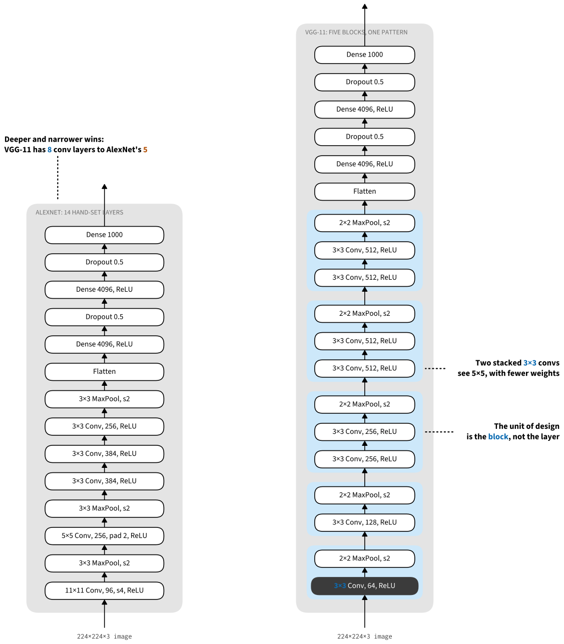
From AlexNet’s hand-tuned layers to VGG’s repeated 3×3 blocks.

Receptive field arithmetic

Why 3×3 only? Stacking small kernels grows the visible patch without paying for a large kernel in one step. For stride 1:

r = 1 + \sum_{i=1}^{L} (k_i - 1).

Two 3×3 convolutions see 1 + 2 + 2 = 5 pixels across: the same receptive field as one 5×5 conv, with 18c^2 instead of 25c^2 weights and one extra ReLU. Deep-and-narrow beats shallow-and-wide.

The VGG block

A reusable subunit: num_convs consecutive Conv-ReLU pairs, then a 2×2 MaxPool:

import tensorflow as tf
from d2l import tensorflow as d2l

def vgg_block(num_convs, num_channels):
    blk = tf.keras.models.Sequential()
    for _ in range(num_convs):
        blk.add(
            tf.keras.layers.Conv2D(num_channels, kernel_size=3,
                                   padding='same', activation='relu'))
    blk.add(tf.keras.layers.MaxPool2D(pool_size=2, strides=2))
    return blk

The VGG network

Five blocks at growing channel counts plus a 3-layer dense head. The “named architecture” is just a tuple of (n_convs, channels) pairs; a different tuple gives VGG-13/16/19:

class VGG(d2l.Classifier):
    def __init__(self, arch, lr=0.1, num_classes=10):
        super().__init__()
        self.save_hyperparameters()
        self.net = tf.keras.models.Sequential()
        for (num_convs, num_channels) in arch:
            self.net.add(vgg_block(num_convs, num_channels))
        self.net.add(
            tf.keras.models.Sequential([
            tf.keras.layers.Flatten(),
            tf.keras.layers.Dense(4096, activation='relu'),
            tf.keras.layers.Dropout(0.5),
            tf.keras.layers.Dense(4096, activation='relu'),
            tf.keras.layers.Dropout(0.5),
            tf.keras.layers.Dense(num_classes)]))

VGG-11 shape check

Each block halves the resolution; channels double until 512:

VGG(arch=((1, 64), (1, 128), (2, 256), (2, 512), (2, 512))).layer_summary(
    (1, 224, 224, 1))

Sequential output shape:     (1, 112, 112, 64)
Sequential output shape:     (1, 56, 56, 128)
Sequential output shape:     (1, 28, 28, 256)
Sequential output shape:     (1, 14, 14, 512)
Sequential output shape:     (1, 7, 7, 512)
Sequential output shape:     (1, 10)

Training a thin VGG

Full VGG-11 is heavy for a notebook, so we thin the channels (16/32/64/128/128) and train on Fashion-MNIST:

trainer = d2l.Trainer(max_epochs=10)
data = d2l.FashionMNIST(batch_size=128, resize=(224, 224))
with d2l.try_gpu():
    model = VGG(arch=((1, 16), (1, 32), (2, 64), (2, 128), (2, 128)), lr=0.01)
    trainer.fit(model, data)

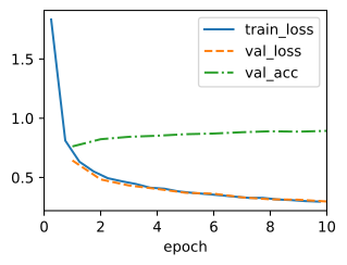
Same pipeline as AlexNet; the block design is what changed.

NiN: 1×1 convolutions and GAP

Network in network (Lin et al., 2013) attacks the FC head: VGG-11’s first dense layer alone needs ~400 MB in FP32.

• 1×1 convolutions: an MLP applied at every pixel; channel mixing and extra nonlinearity at zero spatial cost.
• Global average pooling: one number per channel replaces the giant dense classifier.

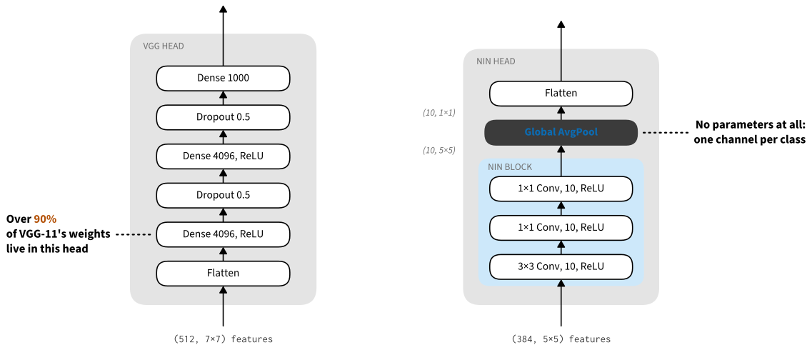
NiN vs. VGG: same body idea, radically different head.

The NiN block

A regular convolution followed by two 1×1 convolutions with ReLUs in between:

def nin_block(out_channels, kernel_size, strides, padding):
    return tf.keras.models.Sequential([
    tf.keras.layers.Conv2D(out_channels, kernel_size, strides=strides,
                           padding=padding),
    tf.keras.layers.Activation('relu'),
    tf.keras.layers.Conv2D(out_channels, 1),
    tf.keras.layers.Activation('relu'),
    tf.keras.layers.Conv2D(out_channels, 1),
    tf.keras.layers.Activation('relu')])

The NiN model

Four NiN blocks (AlexNet’s kernel sizes), max-pool between them, and the last block emits num_classes channels. Then global average pooling. No fully connected layers at all.

class NiN(d2l.Classifier):
    def __init__(self, lr=0.1, num_classes=10):
        super().__init__()
        self.save_hyperparameters()
        self.net = tf.keras.models.Sequential([
            nin_block(96, kernel_size=11, strides=4, padding='valid'),
            tf.keras.layers.MaxPool2D(pool_size=3, strides=2),
            nin_block(256, kernel_size=5, strides=1, padding='same'),
            tf.keras.layers.MaxPool2D(pool_size=3, strides=2),
            nin_block(384, kernel_size=3, strides=1, padding='same'),
            tf.keras.layers.MaxPool2D(pool_size=3, strides=2),
            tf.keras.layers.Dropout(0.5),
            nin_block(num_classes, kernel_size=3, strides=1, padding='same'),
            tf.keras.layers.GlobalAvgPool2D(),
            tf.keras.layers.Flatten()])

NiN shape inspection

Spatial dims shrink, channels grow, and the final block already has one channel per class:

NiN().layer_summary((1, 224, 224, 1))

Sequential output shape:     (1, 54, 54, 96)
MaxPooling2D output shape:   (1, 26, 26, 96)
Sequential output shape:     (1, 26, 26, 256)
MaxPooling2D output shape:   (1, 12, 12, 256)
Sequential output shape:     (1, 12, 12, 384)
MaxPooling2D output shape:   (1, 5, 5, 384)
Dropout output shape:    (1, 5, 5, 384)
Sequential output shape:     (1, 5, 5, 10)
GlobalAveragePooling2D output shape:     (1, 10)
Flatten output shape:    (1, 10)

Training NiN

trainer = d2l.Trainer(max_epochs=10)
data = d2l.FashionMNIST(batch_size=128, resize=(224, 224))
with d2l.try_gpu():
    model = NiN(lr=0.05)
    trainer.fit(model, data)

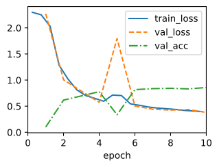
The averaging head costs nothing and does not hurt accuracy; that surprise made GAP the default head ever since.

GoogLeNet: go wide

GoogLeNet (Szegedy et al., 2015) won ImageNet 2014 with two lasting contributions:

• The stem / body / head decomposition of a network, still the universal vocabulary.
• The Inception block: don’t pick a filter size, run 1×1, 3×3, 5×5, and pooling in parallel and concatenate the channels.

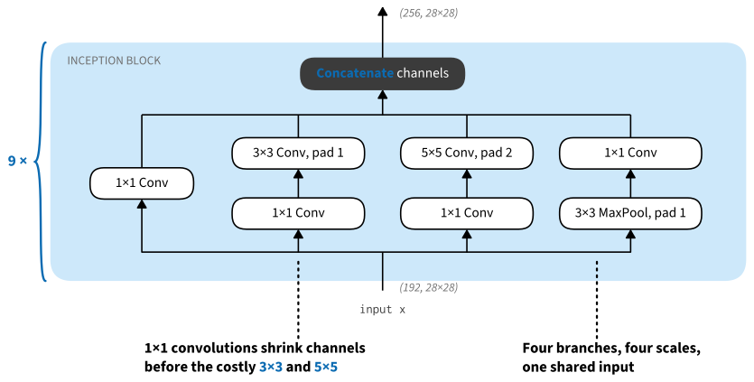
Four branches, four scales, one shared input.

The Inception block in code

Four branches, channel-concatenated; 1×1 convs shrink channels before the costly 3×3 and 5×5:

class Inception(tf.keras.Model):
    # c1--c4 are the number of output channels for each branch
    def __init__(self, c1, c2, c3, c4):
        super().__init__()
        self.b1_1 = tf.keras.layers.Conv2D(c1, 1, activation='relu')
        self.b2_1 = tf.keras.layers.Conv2D(c2[0], 1, activation='relu')
        self.b2_2 = tf.keras.layers.Conv2D(c2[1], 3, padding='same',
                                           activation='relu')
        self.b3_1 = tf.keras.layers.Conv2D(c3[0], 1, activation='relu')
        self.b3_2 = tf.keras.layers.Conv2D(c3[1], 5, padding='same',
                                           activation='relu')
        self.b4_1 = tf.keras.layers.MaxPool2D(3, 1, padding='same')
        self.b4_2 = tf.keras.layers.Conv2D(c4, 1, activation='relu')

    def call(self, x):
        b1 = self.b1_1(x)
        b2 = self.b2_2(self.b2_1(x))
        b3 = self.b3_2(self.b3_1(x))
        b4 = self.b4_2(self.b4_1(x))
        return tf.keras.layers.Concatenate()([b1, b2, b3, b4])

Bottleneck arithmetic

First body block: 192 channels in, 64+128+32+32 = 256 out, spatial size unchanged.

The 5×5 branch, direct: 25 \cdot 192 \cdot 32 \approx 154k weights.

With a 16-channel 1×1 bottleneck first: 192 \cdot 16 + 25 \cdot 16 \cdot 32 \approx 16k, a 10× saving. This trick is in nearly every network since.

The whole network as data

Nine Inception blocks in three groups (2, 5, 2), pooling between groups. The hand-picked channel allocations are just a tuple; assembly is stem + body + head:

arch = (((64, (96, 128), (16, 32), 32), (128, (128, 192), (32, 96), 64)),
        ((192, (96, 208), (16, 48), 64), (160, (112, 224), (24, 64), 64),
         (128, (128, 256), (24, 64), 64), (112, (144, 288), (32, 64), 64),
         (256, (160, 320), (32, 128), 128)),
        ((256, (160, 320), (32, 128), 128), (384, (192, 384), (48, 128), 128)))

class GoogleNet(d2l.Classifier):
    def __init__(self, lr=0.1, num_classes=10):
        super().__init__()
        self.save_hyperparameters()
        pool = lambda: tf.keras.layers.MaxPool2D(pool_size=3, strides=2,
                                                 padding='same')
        stem = tf.keras.Sequential([
            tf.keras.layers.Conv2D(64, 7, strides=2, padding='same',
                                   activation='relu'), pool(),
            tf.keras.layers.Conv2D(64, 1, activation='relu'),
            tf.keras.layers.Conv2D(192, 3, padding='same', activation='relu'),
            pool()])
        body = [tf.keras.Sequential([Inception(*c) for c in group])
                for group in arch]
        head = tf.keras.Sequential([tf.keras.layers.GlobalAvgPool2D(),
                                    tf.keras.layers.Dense(num_classes)])
        self.net = tf.keras.Sequential([stem, body[0], pool(), body[1],
                                        pool(), body[2], head])

Shape check

GoogleNet().layer_summary((1, 96, 96, 1))

Sequential output shape:     (1, 12, 12, 192)
Sequential output shape:     (1, 12, 12, 480)
MaxPooling2D output shape:   (1, 6, 6, 480)
Sequential output shape:     (1, 6, 6, 832)
MaxPooling2D output shape:   (1, 3, 3, 832)
Sequential output shape:     (1, 3, 3, 1024)
Sequential output shape:     (1, 10)

Cheaper than VGG (~7M vs. ~138M parameters) and more accurate: the start of deliberate cost–accuracy design.

What survived

• Blocks (VGG): everything is specified block by block.
• 1×1 convolution (NiN): the standard channel mixer.
• Global average pooling (NiN): the default head.
• Multi-branch (GoogLeNet): survives as grouped convolutions (ResNeXt) and train-time-only branches (RepVGG).
• Inception-style hand-tuned branch cocktails: extinct.

Next ingredient: normalization.