Single Shot Multibox Detection

Single Shot Detection

Single Shot MultiBox Detector (Liu et al., 2016) is the prototype single-stage detector. One forward pass produces class scores and box offsets for every anchor at every scale; NMS keeps the survivors.

The architecture: a CNN trunk, then a pyramid of feature maps at decreasing resolutions. Each level has its own pair of 1×1-style heads — one for class scores, one for box offsets. Predictions from all levels are concatenated.
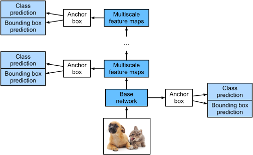
SSD = base network + several multiscale feature blocks; each block has its own anchor predictor.

Scaling to objects in images

Objects appear at different pixel sizes. SSD handles this by predicting from several feature maps at once:

  • early maps: many spatial cells, small receptive fields, small anchor boxes;
  • deeper maps: fewer spatial cells, larger receptive fields, larger anchor boxes.

The model does not resize every candidate region. It learns classification and offset heads at each scale, then pools all anchors into one detection set before NMS.

Class and box prediction heads

For a feature map with a anchors per pixel and q classes, the class head is a 3×3 conv with a(q+1) output channels; the box head outputs 4a:

%matplotlib inline
from d2l import tensorflow as d2l
import tensorflow as tf
from tensorflow import keras
import numpy as np

def cls_predictor(num_anchors, num_classes):
    return keras.layers.Conv2D(num_anchors * (num_classes + 1),
                               kernel_size=3, padding='same')
def bbox_predictor(num_anchors):
    return keras.layers.Conv2D(num_anchors * 4, kernel_size=3, padding='same')

Concatenating across scales

Each level produces predictions of a different shape; flatten and concat them so the loss can run on a single tensor:

def forward(x, block):
    # Keras uses NHWC format; input shape: (N, H, W, C)
    return block(x)

Y1 = forward(tf.zeros((2, 20, 20, 8)), cls_predictor(5, 10))
Y2 = forward(tf.zeros((2, 10, 10, 16)), cls_predictor(3, 10))
Y1.shape, Y2.shape
(TensorShape([2, 20, 20, 55]), TensorShape([2, 10, 10, 33]))
def flatten_pred(pred):
    # pred is (N, H, W, C); flatten H*W*C with channel innermost so that
    # the resulting layout matches multibox_prior's anchor ordering
    return tf.reshape(pred, (tf.shape(pred)[0], -1))

def concat_preds(preds):
    return tf.concat([flatten_pred(p) for p in preds], axis=1)
concat_preds([Y1, Y2]).shape
TensorShape([2, 25300])

Downsampling block

Halves the feature map resolution between scales — two 3×3 conv-BN-ReLU layers + 2×2 max pool:

def down_sample_blk(num_channels):
    blk = keras.Sequential()
    for _ in range(2):
        blk.add(keras.layers.Conv2D(num_channels, kernel_size=3,
                                    padding='same'))
        blk.add(keras.layers.BatchNormalization())
        blk.add(keras.layers.ReLU())
    blk.add(keras.layers.MaxPool2D(pool_size=2, strides=2))
    return blk
forward(tf.zeros((2, 20, 20, 3)), down_sample_blk(10)).shape
TensorShape([2, 10, 10, 10])

Base network

A small CNN that takes the input image down to the first useful resolution:

def base_net():
    blk = keras.Sequential()
    for num_filters in [16, 32, 64]:
        blk.add(down_sample_blk(num_filters))
    return blk

forward(tf.zeros((2, 256, 256, 3)), base_net()).shape
TensorShape([2, 32, 32, 64])

Five-block pyramid

Stack base network + a few downsampling blocks. Each level exposes its feature map for anchor prediction:

def get_blk(i):
    if i == 0:
        return base_net()
    elif i == 4:
        return keras.layers.GlobalMaxPool2D(keepdims=True)
    else:
        return down_sample_blk(128)
def blk_forward(X, blk, size, ratio, cls_predictor, bbox_predictor,
                training=False):
    Y = blk(X, training=training)
    # Keras uses NHWC; multibox_prior expects NCHW (shape[-2:] = H, W)
    Y_nchw = tf.transpose(Y, (0, 3, 1, 2))
    anchors = d2l.multibox_prior(Y_nchw, sizes=size, ratios=ratio)
    # Keep cls_preds and bbox_preds in NHWC; flatten_pred relies on the
    # channel-last memory layout to align with multibox_prior's anchor order
    cls_preds = cls_predictor(Y, training=training)
    bbox_preds = bbox_predictor(Y, training=training)
    return (Y, anchors, cls_preds, bbox_preds)

Per-level scales

Bigger anchor scales at deeper levels (small feature map → large receptive field → large anchors):

  • five feature levels use progressively larger anchors;
  • each level predicts class logits and box offsets;
  • predictions are concatenated across levels before loss or decoding.

TinySSD model

The full model is a feature pyramid plus two lightweight heads per level:

\text{image} \rightarrow \{(\text{anchors}_\ell, \text{class}_\ell, \text{box}_\ell)\}_{\ell=1}^{5}.

Showing the whole class definition on a slide hides the idea; the important contract is the output shape and anchor ordering. Every anchor needs one class vector and one four-number offset vector.

TinySSD output shapes

For a 256 \times 256 image, the five feature maps create (32^2 + 16^2 + 8^2 + 4^2 + 1) \times 4 = 5444 anchors. With one foreground class, expect:

  • anchors: (batch, 5444, 4);
  • class logits: (batch, 5444, 2) for background/banana;
  • offsets: (batch, 5444 * 4).
output anchors: (1, 5444, 4)
output class preds: (32, 5444, 2)
output bbox preds: (32, 21776)

Loading data + init

batch_size = 32
train_iter, _ = d2l.load_data_bananas(batch_size)
read 1000 training examples
read 100 validation examples
net = TinySSD(num_classes=1)
net.compile(optimizer=keras.optimizers.SGD(learning_rate=0.2,
                                           weight_decay=5e-4))

Multi-task loss

Two loss terms:

  • Classification — cross-entropy over class scores.
  • LocalizationL_1 on box offsets, computed only on positive anchors (ignore the rest).

\mathcal{L} = \text{CE}(\hat{\mathbf{c}}, \mathbf{c}) + \frac{1}{N_+}\sum_i m_i \lVert \hat{\mathbf{t}}_i - \mathbf{t}_i\rVert_1,

where m_i=1 only for anchors matched to an object.

# Loss functions are encapsulated in TinySSD._compute_ssd_loss and
# train_step; these module-level helpers mirror the other frameworks for
# use in evaluation after training.
_cls_loss = keras.losses.SparseCategoricalCrossentropy(
    from_logits=True, reduction='none')

def calc_loss(cls_preds, cls_labels, bbox_preds, bbox_labels, bbox_masks):
    batch_size = cls_preds.shape[0]
    num_classes = cls_preds.shape[2]
    # Per-example mean cross-entropy over anchors (shape: (batch_size,))
    cls = tf.reduce_mean(
        tf.reshape(_cls_loss(tf.reshape(cls_labels, [-1]),
                             tf.reshape(cls_preds, [-1, num_classes])),
                   [batch_size, -1]),
        axis=1)
    # Per-example mean L1 bbox loss (shape: (batch_size,)) to match PT/JAX
    bbox = tf.reduce_mean(
        tf.abs((bbox_preds - bbox_labels) * bbox_masks), axis=1)
    return cls + bbox
def cls_eval(cls_preds, cls_labels):
    # Because the class prediction results are on the final dimension,
    # `argmax` needs to specify this dimension
    return float(tf.reduce_sum(
        tf.cast(tf.argmax(cls_preds, axis=-1) ==
                tf.cast(cls_labels, tf.int64), tf.int64)))

def bbox_eval(bbox_preds, bbox_labels, bbox_masks):
    return float(tf.reduce_sum(
        tf.abs((bbox_labels - bbox_preds) * bbox_masks)))

Training

Standard SGD loop, two evaluation metrics (class accuracy, box mean abs error). Read them together: class accuracy is dominated by many background anchors, while box error only makes sense on matched positive anchors.

num_epochs, timer = 20, d2l.Timer()
animator = d2l.Animator(xlabel='epoch', xlim=[1, num_epochs],
                        legend=['class error', 'bbox mae'])
# Anchors depend only on the input *shape*, so for a fixed input size
# they're constant across the epoch. Grab them once here and reuse
# them in every batch's multibox_target call — saves one forward pass
# per step.
sample_features, _ = next(iter(train_iter))
sample_features = tf.cast(sample_features, tf.float32)
anchors_static, _, _ = net(sample_features, training=False)
# `multibox_target` mixes TF ops with NumPy / `.numpy()` calls, which
# can't run inside `@tf.function`. We keep it eager and only put the
# pure-TF gradient step under @tf.function. The wrapper closes over
# `net` so its trainable variables aren't @tf.function arguments
# (which would re-trace each call) — same pattern that worked for
# gan / dcgan.
@tf.function(reduce_retracing=True)
def _grad_step(features, bbox_labels, bbox_masks, cls_labels):
    with tf.GradientTape() as tape:
        _, cls_preds, bbox_preds = net(features, training=True)
        loss = net._compute_ssd_loss(cls_preds, cls_labels, bbox_preds,
                                     bbox_labels, bbox_masks)
    grads = tape.gradient(loss, net.trainable_variables)
    net.optimizer.apply_gradients(zip(grads, net.trainable_variables))
    cls_correct = tf.reduce_sum(
        tf.cast(tf.argmax(cls_preds, axis=-1) ==
                tf.cast(cls_labels, tf.int64), tf.int64))
    cls_total = tf.cast(tf.size(cls_labels), tf.int64)
    bbox_abs = tf.reduce_sum(
        tf.abs((bbox_preds * bbox_masks) - (bbox_labels * bbox_masks)))
    bbox_total = tf.cast(tf.size(bbox_labels), tf.float32)
    return loss, cls_correct, cls_total, bbox_abs, bbox_total
for epoch in range(num_epochs):
    # Accumulate metrics as TF tensors so the inner loop never forces
    # a host sync (the per-batch `int(logs['cls_correct'])` was a
    # significant bottleneck before).
    cls_correct_sum = tf.zeros((), dtype=tf.int64)
    cls_total = tf.zeros((), dtype=tf.int64)
    bbox_abs_total = tf.zeros((), dtype=tf.float32)
    bbox_total = tf.zeros((), dtype=tf.float32)
    for features, target in train_iter:
        timer.start()
        features = tf.cast(features, tf.float32)
        target = tf.cast(target, tf.float32)
        bbox_labels, bbox_masks, cls_labels = d2l.multibox_target(
            anchors_static, target)
        _, cc, ct, ba, bt = _grad_step(features, bbox_labels,
                                       bbox_masks, cls_labels)
        cls_correct_sum += cc
        cls_total += ct
        bbox_abs_total += ba
        bbox_total += bt
    cls_err = float(1 - cls_correct_sum / cls_total)
    bbox_mae = float(bbox_abs_total / bbox_total)
    animator.add(epoch + 1, (cls_err, bbox_mae))
print(f'class err {cls_err:.2e}, bbox mae {bbox_mae:.2e}')
print(f'{len(train_iter) * batch_size / timer.stop():.1f} examples/sec')
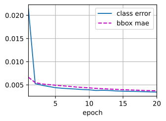
class err 3.46e-03, bbox mae 3.73e-03
1104.0 examples/sec

Inference

Forward pass → anchors + class scores + offsets → invert offsets → NMS → keep boxes above a confidence threshold:

from PIL import Image as PILImage
img_pil = PILImage.open('../img/banana.jpg')
img = np.array(img_pil)
# img is (H, W, C); add batch dim for NHWC input
X = tf.expand_dims(tf.cast(img, tf.float32), axis=0)
def predict(X):
    anchors, cls_preds, bbox_preds = net(X, training=False)
    # cls_preds: (batch, num_anchors, num_classes+1) -> softmax -> transpose
    # to (batch, num_classes+1, num_anchors) for multibox_detection
    cls_probs = tf.transpose(tf.nn.softmax(cls_preds, axis=-1), (0, 2, 1))
    output = d2l.multibox_detection(cls_probs, bbox_preds, anchors)
    # Drop padding rows (class index -1).
    mask = output[0, :, 0] != -1
    idx = tf.where(mask)[:, 0]
    return tf.gather(output[0], idx)

output = predict(X)

Detect bananas

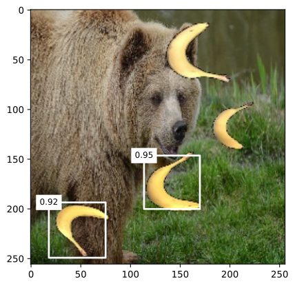
Visualize all predictions with confidence ≥ 0.9. The useful thing to notice is not the raw tensor length, but whether NMS leaves one tight high-confidence box per banana:

def display(img, output, threshold):
    d2l.set_figsize((5, 5))
    fig = d2l.plt.imshow(img)
    for row in output:
        score = float(row[1])
        if score < threshold:
            continue
        h, w = img.shape[:2]
        bbox = [row[2:6] * np.array((w, h, w, h), dtype=np.float32)]
        d2l.show_bboxes(fig.axes, bbox, '%.2f' % score, 'w')

display(img, output, threshold=0.9)
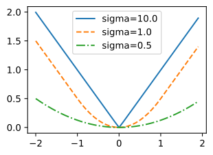
def smooth_l1(data, scalar):
    cond = tf.abs(data) < 1 / (scalar ** 2)
    quad = (scalar * data) ** 2 / 2
    lin = tf.abs(data) - 0.5 / (scalar ** 2)
    return tf.where(cond, quad, lin)

sigmas = [10, 1, 0.5]
lines = ['-', '--', '-.']
x = tf.range(-2.0, 2.0, 0.1)
d2l.set_figsize()

for l, s in zip(lines, sigmas):
    y = smooth_l1(x, scalar=s)
    d2l.plt.plot(x, y, l, label='sigma=%.1f' % s)
d2l.plt.legend();
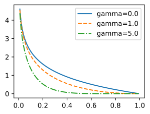
def focal_loss(gamma, x):
    return -(1 - x) ** gamma * tf.math.log(x)

x = tf.range(0.01, 1.0, 0.01)
for l, gamma in zip(lines, [0, 1, 5]):
    y = d2l.plt.plot(x, focal_loss(gamma, x), l, label='gamma=%.1f' % gamma)
d2l.plt.legend();
Recap

  • SSD = base CNN + multiscale feature pyramid + per-level class & offset heads.
  • One forward pass → all anchor predictions; NMS at the end. No region proposal step.
  • Loss = class cross-entropy + offset L_1, only on positive anchors.
  • SSD and RetinaNet are anchor-based dense single-stage detectors. YOLO is a related single-stage family, while modern anchor-free detectors remove explicit anchors but keep dense classification/localization over feature maps.