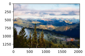
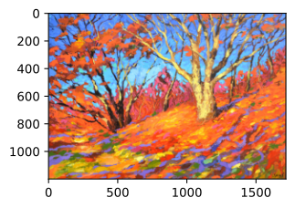
%matplotlib inline
from d2l import tensorflow as d2l
import tensorflow as tf
import keras
import numpy as np
from PIL import Image
d2l.set_figsize()
content_img = Image.open('../img/rainier.jpg')
d2l.plt.imshow(content_img);Neural style transfer (Gatys, Ecker, Bethge 2015): combine the content of one image with the style of another. No model training — just iterative optimization of pixel values against a loss defined over a frozen pretrained CNN.
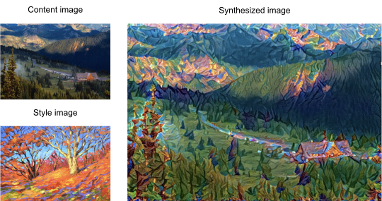
Content + style → synthesized image.
In a pretrained ImageNet CNN:
Define a loss matching both; optimize over the synthesized image’s pixels.
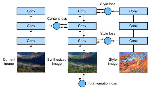
Pipeline: forward pass extracts content + style features; backprop into pixels.
ImageNet mean/std normalization in, inverse on the way out:
# We keep the synthesized image in NCHW layout internally (matching PT/JAX
# so the #@tab-all gram/tv_loss/compute_loss cells work unchanged).
# VGG-19 expects NHWC, so we transpose when calling the feature extractor.
rgb_mean = tf.constant([0.485, 0.456, 0.406], dtype=tf.float32)
rgb_std = tf.constant([0.229, 0.224, 0.225], dtype=tf.float32)
def preprocess(img, image_shape):
img = img.resize((image_shape[1], image_shape[0])) # PIL: (w, h)
img = np.array(img, dtype=np.float32) / 255.0 # (H, W, C)
img = img.transpose(2, 0, 1) # (C, H, W)
img = (img - rgb_mean.numpy().reshape(3, 1, 1)) / rgb_std.numpy().reshape(
3, 1, 1)
return tf.expand_dims(tf.constant(img, dtype=tf.float32), axis=0)
def postprocess(img):
img = img[0].numpy() # (C, H, W)
img = np.clip(img.transpose(1, 2, 0) * rgb_std.numpy() +
rgb_mean.numpy(), 0, 1)
return imgStyle is a multi-scale phenomenon — match it across several VGG-19 layers (Conv1_1, 2_1, 3_1, 4_1, 5_1). Content is matched at one deeper layer (Conv4_2):
# The #@tab-all indices match torchvision's VGG-19 `features` numbering.
# Keras VGG-19 has a different layer order, so we remap.
_torch_to_tf = {0: 1, 5: 4, 10: 7, 19: 12, 25: 15, 28: 17}
style_layers = [_torch_to_tf[i] for i in style_layers]
content_layers = [_torch_to_tf[i] for i in content_layers]
# Build a multi-output feature-extraction model (skips InputLayer at index 0)
_vgg_layers = pretrained_net.layers
net = keras.Model(
inputs=pretrained_net.input,
outputs=[_vgg_layers[i].output
for i in sorted(set(content_layers + style_layers))])def _to_vgg_input(X_nchw):
"""Convert NCHW tensor (ImageNet-normalised) to VGG-19 NHWC input."""
X_nhwc = tf.transpose(X_nchw, (0, 2, 3, 1))
X_raw = (X_nhwc * tf.reshape(rgb_std, (1, 1, 1, 3))
+ tf.reshape(rgb_mean, (1, 1, 1, 3))) * 255.0
return keras.applications.vgg19.preprocess_input(X_raw)
# _sorted_layers maps the sorted output index → original layer index
_sorted_layer_ids = sorted(set(content_layers + style_layers))
def extract_features(X, content_layers, style_layers):
"""Run VGG-19 and return (contents, styles) as NCHW tensors."""
X_vgg = _to_vgg_input(X)
all_outputs = net(X_vgg, training=False) # list of NHWC tensors
# all_outputs[i] corresponds to _sorted_layer_ids[i]
layer_map = {lid: out for lid, out in zip(_sorted_layer_ids, all_outputs)}
contents = [tf.transpose(layer_map[i], (0, 3, 1, 2)) for i in content_layers]
styles = [tf.transpose(layer_map[i], (0, 3, 1, 2)) for i in style_layers]
return contents, stylesdef get_contents(image_shape):
content_X = preprocess(content_img, image_shape)
contents_Y, _ = extract_features(content_X, content_layers, style_layers)
return content_X, contents_Y
def get_styles(image_shape):
style_X = preprocess(style_img, image_shape)
_, styles_Y = extract_features(style_X, content_layers, style_layers)
return style_X, styles_YSquared error between content and synthesized features at the content layer:
Squared error between Gram matrices of features at each style layer. Gram matrix G = F F^\top captures pairwise channel correlations, discarding spatial location:
Penalizes high-frequency noise; keeps the synthesized image smooth:
\mathcal{L} = \alpha\, \mathcal{L}_\text{content} + \beta\, \mathcal{L}_\text{style} + \gamma\, \mathcal{L}_\text{tv}.
The relative weights determine the visual style — high \beta pushes towards painterly, low \beta keeps photorealism.
content_weight, style_weight, tv_weight = 1, 1e4, 10
def compute_loss(X, contents_Y_hat, styles_Y_hat, contents_Y, styles_Y_gram):
# Calculate the content, style, and total variance losses respectively
contents_l = [content_loss(Y_hat, Y) * content_weight for Y_hat, Y in zip(
contents_Y_hat, contents_Y)]
styles_l = [style_loss(Y_hat, Y) * style_weight for Y_hat, Y in zip(
styles_Y_hat, styles_Y_gram)]
tv_l = tv_loss(X) * tv_weight
# Add up all the losses
l = sum(styles_l + contents_l + [tv_l])
return contents_l, styles_l, tv_l, lStart from the content image (or noise — converges slower but works). The synthesized image is the optimization variable; the network parameters are frozen:
def get_inits(X, lr, styles_Y):
# Initialize synthesized image to the content image (NCHW tf.Variable)
gen_img = tf.Variable(tf.cast(X, tf.float32))
lr_schedule = keras.optimizers.schedules.ExponentialDecay(
initial_learning_rate=lr, decay_steps=50, decay_rate=0.8)
trainer = keras.optimizers.Adam(learning_rate=lr_schedule)
styles_Y_gram = [gram(Y) for Y in styles_Y]
return gen_img, styles_Y_gram, trainerAdam (or LBFGS) optimizes the synthesized image itself. The CNN stays frozen; gradients flow through VGG features back to pixels:
def train(X, contents_Y, styles_Y, lr, num_epochs, lr_decay_epoch):
X, styles_Y_gram, trainer = get_inits(X, lr, styles_Y)
animator = d2l.Animator(xlabel='epoch', ylabel='loss',
xlim=[10, num_epochs],
legend=['content', 'style', 'TV'],
ncols=2, figsize=(7, 2.5))
for epoch in range(num_epochs):
with tf.GradientTape() as tape:
contents_Y_hat, styles_Y_hat = extract_features(
X, content_layers, style_layers)
contents_l, styles_l, tv_l, l = compute_loss(
X, contents_Y_hat, styles_Y_hat, contents_Y, styles_Y_gram)
grads = tape.gradient(l, [X])
trainer.apply_gradients(zip(grads, [X]))
if (epoch + 1) % 10 == 0:
animator.axes[1].imshow(postprocess(X))
animator.add(epoch + 1, [float(sum(contents_l)),
float(sum(styles_l)), float(tv_l)])
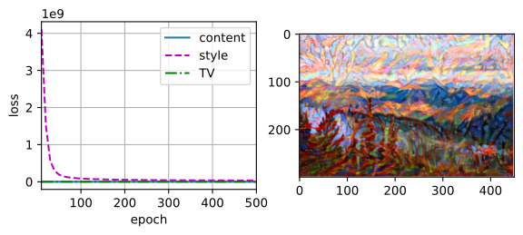
return XAfter a few hundred iterations, the content layout should remain recognizable while colors and local textures move toward the style image. The three plotted losses are weighted differently, so compare their trends rather than their raw magnitudes: