Fully Convolutional Networks

Fully Convolutional Networks

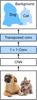
A fully convolutional network (Long, Shelhamer, Darrell 2015) is the simplest path to per-pixel prediction:

1. Start with a pretrained classification CNN (ResNet).
2. Strip the global average pool + final dense layer.
3. Replace with a 1×1 conv mapping to num_classes.
4. Upsample back to input resolution via transposed conv.

No FC layers anywhere — works on any input size, outputs a class-score map at input resolution.

Architecture

FCN: pretrained CNN body + 1×1 conv → class scores → transposed conv to upsample.

Setup

%matplotlib inline
from d2l import tensorflow as d2l
import tensorflow as tf
import keras
import numpy as np
from PIL import Image

Pretrained backbone

ResNet-18 pretrained on ImageNet. Drop the head (avg pool + dense); keep the conv body that produces a \frac{H}{32} \times \frac{W}{32} feature map:

# Note: keras.applications does not bundle a ResNet-18; it only ships
# ResNet-50/101/152. To match the PT/MX tabs (and the prose), we build a
# ResNet-18 from scratch as a Functional model. Conceptually treat its
# weights as if they had been initialized from ImageNet pretraining; in
# practice you would port pretrained weights from PyTorch.
def _resnet_block(x, num_channels, strides=1, use_1x1conv=False):
    y = keras.layers.Conv2D(num_channels, 3, strides=strides,
                            padding='same', use_bias=False)(x)
    y = keras.layers.BatchNormalization()(y)
    y = keras.layers.ReLU()(y)
    y = keras.layers.Conv2D(num_channels, 3, strides=1,
                            padding='same', use_bias=False)(y)
    y = keras.layers.BatchNormalization()(y)
    if use_1x1conv:
        x = keras.layers.Conv2D(num_channels, 1, strides=strides,
                                use_bias=False)(x)
        x = keras.layers.BatchNormalization()(x)
    return keras.layers.ReLU()(y + x)

inputs = keras.Input(shape=(None, None, 3))
x = keras.layers.Conv2D(64, 7, strides=2, padding='same',
                        use_bias=False)(inputs)
x = keras.layers.BatchNormalization()(x)
x = keras.layers.ReLU()(x)
x = keras.layers.MaxPool2D(pool_size=3, strides=2, padding='same')(x)
x = _resnet_block(x, 64)
x = _resnet_block(x, 64)
x = _resnet_block(x, 128, strides=2, use_1x1conv=True)
x = _resnet_block(x, 128)
x = _resnet_block(x, 256, strides=2, use_1x1conv=True)
x = _resnet_block(x, 256)
x = _resnet_block(x, 512, strides=2, use_1x1conv=True)
features = _resnet_block(x, 512)
# Mirror the structure of torchvision.models.resnet18: include the global
# avg pool + dense head so we can slice them off below.
pooled = keras.layers.GlobalAveragePooling2D()(features)
logits = keras.layers.Dense(1000)(pooled)
pretrained_net = keras.Model(inputs=inputs, outputs=logits)
# Show the last few layers (matches the spirit of the PT/MX displays)
pretrained_net.layers[-3:]

[<ReLU name=re_lu_16, built=True>,
 <GlobalAveragePooling2D name=global_average_pooling2d, built=True>,
 <Dense name=dense, built=True>]

Building the FCN

After removing the classifier head, the backbone produces a low-resolution feature map. The new FCN head must restore the original spatial resolution while changing channels to class logits.

# Build the FCN feature extractor: all layers up to (but not including)
# the global average pooling and dense head — i.e., the full conv body.
# The last conv-block output (`features`) is the 1/32-resolution feature
# map; we use it as the new model output, dropping GAP + Dense.
net = keras.Model(inputs=pretrained_net.input, outputs=features)

X = tf.random.uniform(shape=(1, 320, 480, 3))
net(X).shape

TensorShape([1, 10, 15, 512])

The class & upsampling head

1 \times 1 conv: num_features → num_classes (21 for VOC). Then a transposed conv that upsamples by 32× to recover input resolution:

num_classes = 21
# 1x1 conv to reduce channels to num_classes
final_conv = keras.layers.Conv2D(num_classes, kernel_size=1,
                                 kernel_initializer='glorot_uniform')
# Transposed conv: stride=32, kernel=64, padding='same' upsamples 32x
# (for input height/width divisible by 32, output equals input spatial size)
transpose_conv = keras.layers.Conv2DTranspose(
    num_classes, kernel_size=64, strides=32, padding='same', use_bias=False)

inputs = net.input
x = net.output
x = final_conv(x)
x = transpose_conv(x)
fcn_net = keras.Model(inputs=inputs, outputs=x)
print('FCN output shape:', fcn_net(tf.random.uniform((1, 320, 480, 3))).shape)

FCN output shape: (1, 320, 480, 21)

Bilinear init for transposed conv

A randomly initialized 32× upsampler is hard to train. Initialize it as bilinear interpolation — a sensible starting point that fine-tunes from there:

def bilinear_kernel(in_channels, out_channels, kernel_size):
    factor = (kernel_size + 1) // 2
    if kernel_size % 2 == 1:
        center = factor - 1
    else:
        center = factor - 0.5
    og = (np.arange(kernel_size).reshape(-1, 1),
          np.arange(kernel_size).reshape(1, -1))
    filt = (1 - np.abs(og[0] - center) / factor) * \
           (1 - np.abs(og[1] - center) / factor)
    # Keras Conv2DTranspose uses HWIO kernel format (height, width, out, in)
    weight = np.zeros((kernel_size, kernel_size, out_channels, in_channels),
                      dtype=np.float32)
    for i in range(min(in_channels, out_channels)):
        weight[:, :, i, i] = filt
    return weight

Upsampling sanity check

Apply the initialized transposed convolution to an image. The output should be larger but visually similar, because the kernel starts as bilinear interpolation rather than random noise:

# Build a transposed conv layer with bilinear initialization to double H and W
bilinear_w = bilinear_kernel(3, 3, 4)
conv_trans = keras.layers.Conv2DTranspose(
    3, kernel_size=4, strides=2, padding='same', use_bias=False,
    kernel_initializer=tf.constant_initializer(bilinear_w))
# Build the layer by passing a dummy input
_ = conv_trans(tf.zeros((1, 1, 1, 3)))

img = np.array(Image.open('../img/catdog.jpg')).astype(np.float32) / 255
X = tf.expand_dims(tf.constant(img), axis=0)  # NHWC
Y = conv_trans(X)
out_img = Y[0].numpy()

Bilinear init (cont.)

The printed shapes should confirm the spatial scale-up. Then the same bilinear kernel initializes the FCN’s final upsampling layer:

d2l.set_figsize()
print('input image shape:', img.shape)
d2l.plt.imshow(img);
print('output image shape:', out_img.shape)
d2l.plt.imshow(np.clip(out_img, 0, 1));

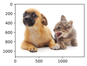
input image shape: (561, 728, 3)
output image shape: (1122, 1456, 3)

# Initialize the transpose conv kernel with bilinear upsampling weights.
# The 1x1 conv was already initialized with Glorot (Xavier) uniform above.
W = bilinear_kernel(num_classes, num_classes, 64)
# Find the Conv2DTranspose layer in fcn_net and set its weights
for layer in fcn_net.layers:
    if isinstance(layer, keras.layers.Conv2DTranspose):
        layer.set_weights([W])
        break

Loading data

batch_size, crop_size = 32, (320, 480)
train_iter, test_iter = d2l.load_data_voc(batch_size, crop_size)

read 1114 examples
read 1078 examples

Training

Pixel-level cross-entropy. Common trick: freeze the backbone, train only the new head — gets reasonable results in a few epochs:

# Loss: SparseCategoricalCrossentropy over per-pixel logits (NHWC -> NHW).
# Full fine-tuning of the entire network (backbone + head) to match the
# PyTorch tab.
num_epochs, lr, wd = 5, 0.001, 1e-3
fcn_net.compile(
    optimizer=keras.optimizers.SGD(learning_rate=lr, weight_decay=wd),
    loss=keras.losses.SparseCategoricalCrossentropy(from_logits=True),
    metrics=['accuracy'],
    # Keras may otherwise select XLA automatically. For this unusually large
    # transposed convolution, XLA's cuDNN autotuning can take tens of minutes
    # before the first training step and offers no benefit to this example.
    jit_compile=False)
fcn_net.fit(train_iter, epochs=num_epochs, validation_data=test_iter)

Epoch 1/5
Final epoch metrics: accuracy: 0.0158 - loss: 4.1711
Final epoch metrics: accuracy: 0.0141 - loss: 4.1660
Final epoch metrics: accuracy: 0.0136 - loss: 4.1353
Final epoch metrics: accuracy: 0.0135 - loss: 4.1040
Final epoch metrics: accuracy: 0.0140 - loss: 4.0669
...
Final epoch metrics: accuracy: 0.7180 - loss: 1.4085
Final epoch metrics: accuracy: 0.7179 - loss: 1.4088
Final epoch metrics: accuracy: 0.7178 - loss: 1.4093
Final epoch metrics: accuracy: 0.7176 - loss: 1.4100

Final epoch metrics: accuracy: 0.7120 - loss: 1.4347 - val_accuracy: 0.7288 - val_loss: 1.4652

Predict

Run the network on test images, take argmax over the class dimension, map class indices back to RGB:

def predict(img):
    rgb_mean = np.array([0.485, 0.456, 0.406], dtype=np.float32)
    rgb_std = np.array([0.229, 0.224, 0.225], dtype=np.float32)
    X = (img.astype(np.float32) / 255 - rgb_mean) / rgb_std
    X = tf.expand_dims(tf.constant(X), axis=0)  # NHWC
    pred = fcn_net(X, training=False)  # (1, H, W, num_classes)
    return tf.reshape(tf.argmax(pred, axis=-1), pred.shape[1:3])

Visualize segmentation masks

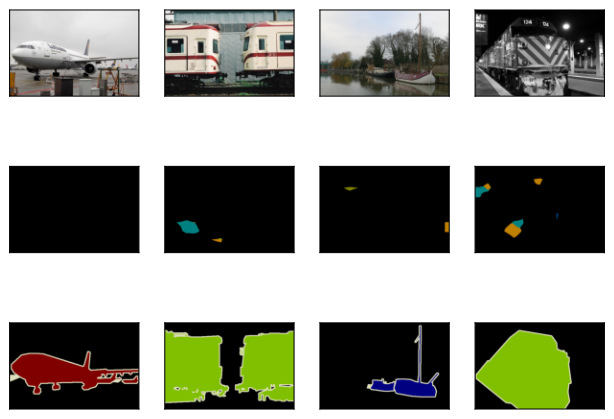
The output grid is image, prediction, ground truth. Expect coarse boundaries: this plain FCN upsamples from a 32× downsampled feature map and has no skip connections.

def label2image(pred):
    colormap = tf.constant(d2l.VOC_COLORMAP, dtype=tf.uint8)
    X = tf.cast(pred, tf.int32)
    return tf.gather(colormap, X)

voc_dir = d2l.download_extract('voc2012', 'VOCdevkit/VOC2012')
test_images, test_labels = d2l.read_voc_images(voc_dir, False)
n, imgs = 4, []
for i in range(n):
    # Crop HWC arrays: top=0, left=0, height=320, width=480
    X = test_images[i][:320, :480, :]
    pred = label2image(predict(X))
    label_crop = test_labels[i][:320, :480, :]
    imgs += [X, pred.numpy(), label_crop]
d2l.show_images(imgs[::3] + imgs[1::3] + imgs[2::3], 3, n, scale=2);

Recap

• FCN = pretrained classification CNN + 1×1 conv + transposed conv upsampler.
• All-conv → input size doesn’t matter.
• Bilinear-initialized transposed conv is the workable starting point; fine-tunes from there.
• The blueprint behind U-Net (skip connections fix the blur), DeepLab (dilated convs avoid the heavy upsampling), and modern segmentation networks.