Compilers and Interpreters

From Eager to Graph Execution

PyTorch / MXNet imperative — eager execution. Every line of Python issues a kernel and waits. Easy to debug, but costs you Python-loop overhead and prevents whole-graph optimization.

The fix: trace or script the model into a graph, then let the framework JIT-compile it (TorchScript, MXNet Hybridize, TF @tf.function, JAX jit). Result: 10–100× less Python overhead, plus operator fusion and memory-layout optimization.

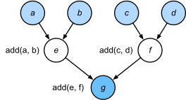
Imperative execution: each line dispatches a separate kernel.

def add(a, b):
    return a + b

def fancy_func(a, b, c, d):
    e = add(a, b)
    f = add(c, d)
    g = add(e, f)
    return g

print(fancy_func(1, 2, 3, 4))

10

Imperative vs symbolic

Imperative: Python-controlled, easy to print/debug, expensive per op. Symbolic: graph captured, compiled once, runs as fused kernels. Modern frameworks let you switch between modes:

def add_():
    return '''
def add(a, b):
    return a + b
'''

def fancy_func_():
    return '''
def fancy_func(a, b, c, d):
    e = add(a, b)
    f = add(c, d)
    g = add(e, f)
    return g
'''

def evoke_():
    return add_() + fancy_func_() + 'print(fancy_func(1, 2, 3, 4))'

prog = evoke_()
print(prog)
y = compile(prog, '', 'exec')
exec(y)

def add(a, b):
    return a + b

def fancy_func(a, b, c, d):
    e = add(a, b)
    f = add(c, d)
    g = add(e, f)
    return g
print(fancy_func(1, 2, 3, 4))
10

Hybridizing a Sequential model

Build the same MLP as a regular module, then opt into graph mode (PyTorch: torch.jit.script; MXNet: HybridSequential.hybridize(); TF: @tf.function):

from d2l import tensorflow as d2l
import tensorflow as tf
from tensorflow.keras.layers import Dense

# Factory for networks
def get_net():
    net = tf.keras.Sequential()
    net.add(tf.keras.Input(shape=(512,)))
    net.add(Dense(256, activation = "relu"))
    net.add(Dense(128, activation = "relu"))
    net.add(Dense(2))
    return net

x = tf.random.normal([1,512])
net = get_net()
net(x)

<tf.Tensor: shape=(1, 2), dtype=float32, numpy=array([[-2.119575 ,  0.8965409]], dtype=float32)>

net = tf.function(net)
net(x)

<tf.Tensor: shape=(1, 2), dtype=float32, numpy=array([[-2.119575  ,  0.89654076]], dtype=float32)>

Speedup

Wall-clock benchmark, eager vs hybridized. The exact ratio depends on model size and op count, but the win is usually substantial:

class Benchmark:
    """For measuring running time."""
    def __init__(self, description='Done'):
        self.description = description

    def __enter__(self):
        self.timer = d2l.Timer()
        return self

    def __exit__(self, *args):
        print(f'{self.description}: {self.timer.stop():.4f} sec')

net = get_net()
with Benchmark('Eager Mode'):
    for i in range(1000): net(x)

net = tf.function(net)
with Benchmark('Graph Mode'):
    for i in range(1000): net(x)

Eager Mode: 2.0256 sec
Graph Mode: 0.8512 sec

Serialization

A graph is portable: save it once, load and run from C++, mobile, or another language without Python in the loop. Models in production almost always ship the graph form:

net = get_net()
tf.saved_model.save(net, 'my_mlp')
!ls -lh my_mlp*

Inspecting the graph

The compiled module exposes its computation graph for inspection (or further optimization):

Recap

• Eager Python is great for development; graph form is faster for production.
• Hybridization = trace or script imperative code into a static graph, then JIT-compile.
• Wins: kernel fusion, no Python overhead, deployable to C++ / mobile.
• Costs: control flow that depends on tensor values is harder to capture; debugging is less interactive.