Self-attention as MultiHead(X, X, X)

Self-Attention and Positional Encoding

Self-Attention

Bahdanau attention links two sequences (decoder steps to encoder steps). What if we use the same trick within a single sequence — let every token query every other token? That’s self-attention: queries, keys, and values all come from the same input.

The output for each token is a weighted average of all tokens, with weights determined by query-key compatibility. This is the elementary block of every Transformer encoder and decoder layer.

from d2l import tensorflow as d2l
import numpy as np
import tensorflow as tf

Reuse multi-head attention with the same input fed three times. Output shape matches input shape — same sequence length, same hidden size:

num_hiddens, num_heads = 100, 5
attention = d2l.MultiHeadAttention(num_hiddens, num_hiddens, num_hiddens,
                                   num_hiddens, num_heads, 0.5)

Shape check:

batch_size, num_queries, valid_lens = 2, 4, tf.constant([3, 2])
X = tf.ones((batch_size, num_queries, num_hiddens))
d2l.check_shape(attention(X, X, X, valid_lens, training=False),
                (batch_size, num_queries, num_hiddens))

CNN vs. RNN vs. self-attention

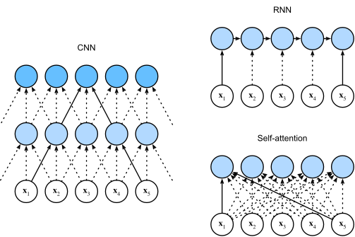
Three ways to map a length-n sequence to another length-n sequence with d-dim tokens:

Compute Sequential ops Max path
CNN (k-wide) \mathcal{O}(knd^2) \mathcal{O}(1) \mathcal{O}(n/k)
RNN \mathcal{O}(nd^2) \mathcal{O}(n) \mathcal{O}(n)
Self-attention \mathcal{O}(n^2 d) \mathcal{O}(1) \mathcal{O}(1)

Self-attention wins on parallelism and path length — every token reaches every other in one hop. The price is n^2 scaling.

One picture

CNN, RNN, self-attention. Path lengths: \mathcal{O}(n/k), \mathcal{O}(n), \mathcal{O}(1).

Why we need positional encoding

Self-attention is permutation-equivariant: shuffle the input tokens, and the outputs shuffle the same way. The model has no idea about word order.

Solution: inject position information into each token’s representation. Vaswani et al. use fixed sine/cosine encodings:

p_{i,2j} = \sin\!\left(\frac{i}{10000^{2j/d}}\right),\quad p_{i,2j+1} = \cos\!\left(\frac{i}{10000^{2j/d}}\right).

Different frequencies along the embedding dimension; same position i across all dims gives a unique fingerprint.

PositionalEncoding class

Precompute \mathbf{P} once for max_len positions, slice to actual length at forward time, add to inputs:

class PositionalEncoding(tf.keras.layers.Layer):
    """Positional encoding."""
    def __init__(self, num_hiddens, dropout, max_len=1000):
        super().__init__()
        self.dropout = tf.keras.layers.Dropout(dropout)
        # Create a long enough P
        self.P = np.zeros((1, max_len, num_hiddens))
        X = np.arange(max_len, dtype=np.float32).reshape(
            -1,1)/np.power(10000, np.arange(
            0, num_hiddens, 2, dtype=np.float32) / num_hiddens)
        self.P[:, :, 0::2] = np.sin(X)
        self.P[:, :, 1::2] = np.cos(X[:, :num_hiddens // 2])
        
    def call(self, X, training=False, **kwargs):
        X = X + self.P[:, :X.shape[1], :]
        return self.dropout(X, training=training)

Frequency along the dimension

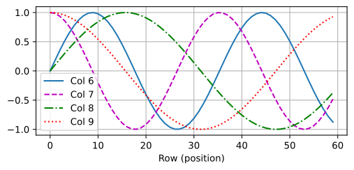
Plot four columns of \mathbf{P}. Lower-index columns oscillate fast; higher columns oscillate slow:

encoding_dim, num_steps = 32, 60
pos_encoding = PositionalEncoding(encoding_dim, 0)
X = pos_encoding(tf.zeros((1, num_steps, encoding_dim)), training=False)
P = pos_encoding.P[:, :X.shape[1], :]
d2l.plot(np.arange(num_steps), P[0, :, 6:10].T, xlabel='Row (position)',
         figsize=(6, 2.5), legend=["Col %d" % d for d in range(6, 10)])

Position as continuous binary

Compare with binary representations of small integers — same “low bits flip fast, high bits flip slow” pattern, but in continuous values:

for i in range(8):
    print(f'{i} in binary is {i:>03b}')
0 in binary is 000
1 in binary is 001
2 in binary is 010
3 in binary is 011
4 in binary is 100
5 in binary is 101
6 in binary is 110
7 in binary is 111

The full positional matrix

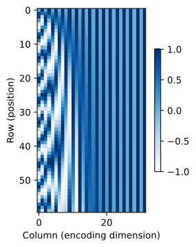
Heatmap reveals the multi-frequency structure. Each row is a unique fingerprint for a position:

P = tf.expand_dims(tf.expand_dims(P[0, :, :], axis=0), axis=0)
d2l.show_heatmaps(P, xlabel='Column (encoding dimension)',
                  ylabel='Row (position)', figsize=(3.5, 4), cmap='Blues')

Why sin/cos: relative positions

For any fixed offset \delta, the encoding at position i + \delta is a linear function of the encoding at position i:

\begin{bmatrix} p_{i+\delta, 2j} \\ p_{i+\delta, 2j+1} \end{bmatrix} = \begin{bmatrix} \cos(\delta\omega_j) & \sin(\delta\omega_j) \\ -\sin(\delta\omega_j) & \cos(\delta\omega_j) \end{bmatrix} \begin{bmatrix} p_{i, 2j} \\ p_{i, 2j+1} \end{bmatrix}.

The rotation depends on \delta but not on i. So the network can learn to “shift attention by 5 tokens” with one linear transformation — relative positions come for free.
Recap

  • Self-attention = multi-head attention with \mathbf{Q} = \mathbf{K} = \mathbf{V} = \mathbf{X}.
  • Output sequence length = input sequence length.
  • Compared to RNNs: same complexity per step but \mathcal{O}(1) path length and full parallelism. Cost: \mathcal{O}(n^2 d).
  • Self-attention is permutation-equivariant; need positional encoding to know token order.
  • Sin/cos encoding gives unique absolute positions and lets the model express relative offsets as linear maps.