Looking at the data

Naive Bayes

Naive Bayes Classification

Naive Bayes — the simplest probabilistic classifier. Apply Bayes’ rule:

P(y \mid \mathbf{x}) \propto P(y) \prod_i P(x_i \mid y).

The “naive” part is the assumption that features are conditionally independent given the class. Wrong in general — pixels of an image are obviously correlated — but the model is fast, requires little data, and is a useful starting point.

This deck applies it to MNIST digit classification with binarized pixels.

Setup + binary MNIST

Binarize pixels so each pixel can be modeled as a Bernoulli random variable conditioned on the digit class.

%matplotlib inline
from d2l import tensorflow as d2l
import math
import tensorflow as tf
d2l.use_svg_display()

Inspect the binarized digits before fitting: the class templates are recognizable, but neighboring pixels are clearly dependent.

((train_images, train_labels), (
    test_images, test_labels)) = tf.keras.datasets.mnist.load_data()

# Original pixel values of MNIST range from 0-255 (as the digits are stored as
# uint8). For this section, pixel values that are greater than 128 (in the
# original image) are converted to 1 and values that are less than 128 are
# converted to 0. See section 18.9.2 and 18.9.3 for why
train_images = tf.floor(tf.constant(train_images / 128, dtype = tf.float32))
test_images = tf.floor(tf.constant(test_images / 128, dtype = tf.float32))

train_labels = tf.constant(train_labels, dtype = tf.int32)
test_labels = tf.constant(test_labels, dtype = tf.int32)

image, label = train_images[2], train_labels[2]
image.shape, label.numpy()

(TensorShape([28, 28]), np.int32(4))

image.shape, image.dtype

(TensorShape([28, 28]), tf.float32)

Per-class pixel statistics

For each class y and pixel i, estimate P(x_i = 1 \mid y) from the training set. With Laplace smoothing to avoid zeros:

label.numpy(), label.dtype

(np.int32(4), tf.int32)

images = tf.stack([train_images[i] for i in range(10, 38)], axis=0)
labels = tf.constant([train_labels[i].numpy() for i in range(10, 38)])
images.shape, labels.shape

(TensorShape([28, 28, 28]), TensorShape([28]))

d2l.show_images(images, 2, 9);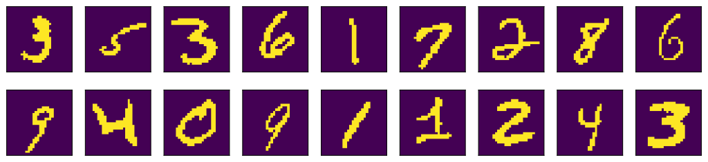

Training: just count

Training is counting, not gradient descent: estimate class priors and per-pixel likelihoods directly from the labeled examples.

X = train_images
Y = train_labels

n_y = tf.Variable(tf.zeros(10))
for y in range(10):
    n_y[y].assign(tf.reduce_sum(tf.cast(Y == y, tf.float32)))
P_y = n_y / tf.reduce_sum(n_y)
P_y

<tf.Tensor: shape=(10,), dtype=float32, numpy=
array([0.09871667, 0.11236667, 0.0993    , 0.10218333, 0.09736667,
       0.09035   , 0.09863333, 0.10441667, 0.09751666, 0.09915   ],
      dtype=float32)>

n_x = tf.Variable(tf.zeros((10, 28, 28)))
for y in range(10):
    n_x[y].assign(tf.cast(tf.reduce_sum(
        X.numpy()[Y.numpy() == y], axis=0), tf.float32))
P_xy = (n_x + 1) / tf.reshape((n_y + 2), (10, 1, 1))

d2l.show_images(P_xy, 2, 5);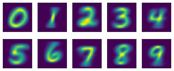

Training (cont.)

Training stores only class priors and per-class pixel probabilities; prediction multiplies those likelihood terms, usually in log-space.

def bayes_pred(x):
    x = tf.expand_dims(x, axis=0)  # (28, 28) -> (1, 28, 28)
    p_xy = P_xy * x + (1 - P_xy)*(1 - x)
    p_xy = tf.math.reduce_prod(tf.reshape(p_xy, (10, -1)), axis=1)  # p(x|y)
    return p_xy * P_y

image, label = test_images[0], test_labels[0]
bayes_pred(image)

<tf.Tensor: shape=(10,), dtype=float32, numpy=array([0., 0., 0., 0., 0., 0., 0., 0., 0., 0.], dtype=float32)>

a = 0.1
print('underflow:', a**784)
print('logarithm is normal:', 784*tf.math.log(a).numpy())

underflow: 0.0
logarithm is normal: -1805.2267

Predicting in log-space

Sums of logs instead of products of probabilities — avoids underflow:

log_P_xy = tf.math.log(P_xy)
log_P_xy_neg = tf.math.log(1 - P_xy)
log_P_y = tf.math.log(P_y)

def bayes_pred_stable(x):
    x = tf.expand_dims(x, axis=0)  # (28, 28) -> (1, 28, 28)
    p_xy = log_P_xy * x + log_P_xy_neg * (1 - x)
    p_xy = tf.math.reduce_sum(tf.reshape(p_xy, (10, -1)), axis=1)  # p(x|y)
    return p_xy + log_P_y

py = bayes_pred_stable(image)
py

<tf.Tensor: shape=(10,), dtype=float32, numpy=
array([-268.9725  , -301.7044  , -245.19516 , -218.87387 , -193.45705 ,
       -206.0909  , -292.52264 , -114.625656, -220.33133 , -163.17844 ],
      dtype=float32)>

tf.argmax(py, axis=0, output_type = tf.int32) == label

<tf.Tensor: shape=(), dtype=bool, numpy=True>

Evaluating

The accuracy is useful mostly as a sanity check: on images, the conditional-independence assumption leaves visible performance on the table.

def predict(X):
    return [tf.argmax(
        bayes_pred_stable(x), axis=0, output_type = tf.int32).numpy()
            for x in X]

X = tf.stack([test_images[i] for i in range(10, 38)], axis=0)
y = tf.constant([test_labels[i].numpy() for i in range(10, 38)])
preds = predict(X)
d2l.show_images(X, 2, 9, titles=[str(d) for d in preds]);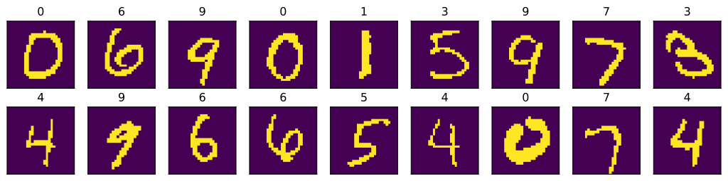

X = test_images
y = test_labels
preds = tf.constant(predict(X), dtype=tf.int32)
# Validation accuracy
tf.reduce_sum(tf.cast(preds == y, tf.float32)).numpy() / len(y)

np.float32(0.8427)

Recap

• Bayes rule + conditional independence = naive Bayes.
• Training is one pass over the data — count and smooth.
• Surprisingly competitive baseline for text classification (sparse features, large vocab).
• Bad on images (independence is too wrong) — but a great teaching example for Bayesian classification.