Eigendecompositions

Eigenvectors and Dynamics

A square matrix \mathbf{A} has eigenvalue \lambda and eigenvector \mathbf{v} when

\mathbf{A}\mathbf{v} = \lambda \mathbf{v}.

Geometrically: \mathbf{A} stretches \mathbf{v} by \lambda but doesn’t rotate it. If \mathbf{A} is diagonalizable: \mathbf{A} = \mathbf{V}\mathbf{\Lambda}\mathbf{V}^{-1} — a basis change in which the action is just stretching along axes.

Why we care: matrix powers \mathbf{A}^t are governed by \lambda^t. Repeated application of \mathbf{A} aligns arbitrary inputs with the dominant eigenvector. That’s the heart of vanishing/exploding gradients in RNNs, of PageRank, and of every iterative solver.

A concrete example

Use a small matrix so the geometry is visible: applying \mathbf{A} to an eigenvector changes scale but not direction.

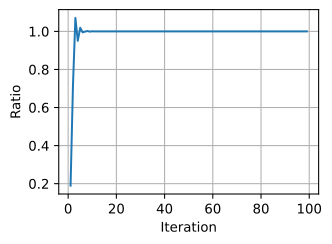
%matplotlib inline
from d2l import tensorflow as d2l
from IPython import display
import tensorflow as tf

tf.linalg.eig(tf.constant([[2, 1], [2, 3]], dtype=tf.float64))

(<tf.Tensor: shape=(2,), dtype=complex128, numpy=array([1.+0.j, 4.+0.j])>,
 <tf.Tensor: shape=(2, 2), dtype=complex128, numpy=
 array([[-0.70710678+0.j, -0.4472136 +0.j],
        [ 0.70710678+0.j, -0.89442719+0.j]])>)

Gershgorin circles

Cheap eigenvalue bounds without computing them: eigenvalues lie in the union of disks centered at a_{ii} with radius \sum_{j \ne i} |a_{ij}|. Useful for stability arguments:

A = tf.constant([[1.0, 0.1, 0.1, 0.1],
                [0.1, 3.0, 0.2, 0.3],
                [0.1, 0.2, 5.0, 0.5],
                [0.1, 0.3, 0.5, 9.0]])

v, _ = tf.linalg.eigh(A)
v

<tf.Tensor: shape=(4,), dtype=float32, numpy=array([0.99228525, 2.9734395 , 4.953943  , 9.080336  ], dtype=float32)>

Eigenvectors govern long-run behavior

Power iteration: keep multiplying by \mathbf{A}. The direction converges to the leading eigenvector; the norm grows like \lambda_1^t:

k = 5
A = tf.random.normal((k, k), dtype=tf.float64)
A

<tf.Tensor: shape=(5, 5), dtype=float64, numpy=
array([[ 1.03149539,  0.41232531,  0.02266882,  0.67373294, -0.87260178],
       [-1.0966355 , -0.39447736,  0.57244043, -0.51296719, -0.33833431],
       [-0.44988705, -1.01188798, -1.66646424, -1.84863467, -0.63040954],
       [ 1.25508111, -1.64698523,  0.89168499,  0.8669014 ,  0.09465951],
       [ 1.191481  , -1.45418164,  0.21448572,  0.80032122,  1.53658541]])>

# Calculate the sequence of norms after repeatedly applying `A`
v_in = tf.random.normal((k, 1), dtype=tf.float64)

norm_list = [tf.norm(v_in).numpy()]
for i in range(1, 100):
    v_in = tf.matmul(A, v_in)
    norm_list.append(tf.norm(v_in).numpy())

d2l.plot(tf.range(0, 100), norm_list, 'Iteration', 'Value')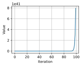

# Compute the scaling factor of the norms
norm_ratio_list = []
for i in range(1, 100):
    norm_ratio_list.append(norm_list[i]/norm_list[i - 1])

d2l.plot(tf.range(1, 100), norm_ratio_list, 'Iteration', 'Ratio')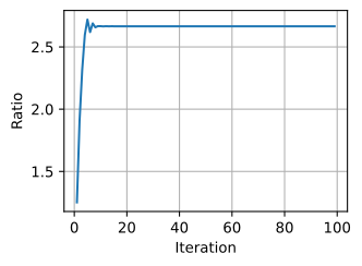

Relating back

After repeated multiplication, normalize the vector to read off the direction; the scale factor estimates the dominant eigenvalue.

# Compute the eigenvalues (A is not symmetric in general, so use eig).
eigs = tf.linalg.eig(A)[0].numpy().tolist()
norm_eigs = [abs(x) for x in eigs]
norm_eigs.sort()
print(f'norms of eigenvalues: {norm_eigs}')

norms of eigenvalues: [0.05364470876910993, 1.8603626913408091, 1.8603626913408091, 2.2231936803962955, 2.2231936803962955]

# Rescale the matrix `A`
A /= norm_eigs[-1]

# Do the same experiment again
v_in = tf.random.normal((k, 1), dtype=tf.float64)

norm_list = [tf.norm(v_in).numpy()]
for i in range(1, 100):
    v_in = tf.matmul(A, v_in)
    norm_list.append(tf.norm(v_in).numpy())

d2l.plot(tf.range(0, 100), norm_list, 'Iteration', 'Value')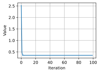

# Also plot the ratio
norm_ratio_list = []
for i in range(1, 100):
    norm_ratio_list.append(norm_list[i]/norm_list[i-1])

d2l.plot(tf.range(1, 100), norm_ratio_list, 'Iteration', 'Ratio')

Recap

• \mathbf{A}\mathbf{v} = \lambda \mathbf{v}: \mathbf{A} acts as scaling along the eigenvector axes.
• Largest |\lambda| controls long-run iterated dynamics.
• Symmetric matrices have orthonormal eigenvectors and real eigenvalues — the basis for PCA.
• Vanishing/exploding RNN gradients = “iterated map” with bad spectral radius.