Bernoulli

Distributions

Common Probability Distributions

A reference tour of the distributions used throughout the book — what they look like, when they apply, and how to sample / evaluate them in code.

• Bernoulli — single coin flip; binary classification conditional.
• Discrete uniform — equiprobable categories.
• Continuous uniform — random initialization, dropout masks (in expectation).
• Binomial — count of successes in n Bernoullis.
• Poisson — rare events count; CTR distributions, click counts.
• Gaussian — by far the most-used; CLT, regression noise model, default prior.

Setup

Imports and plotting helpers are shared across the PMF, PDF, CDF, and sampling examples below.

%matplotlib inline
from d2l import tensorflow as d2l
from IPython import display
from math import erf, factorial
import tensorflow as tf
import tensorflow_probability as tfp

tf.pi = tf.acos(tf.zeros(1)) * 2  # Define pi in TensorFlow

P(X=1) = p, P(X=0) = 1-p. Mean p, variance p(1-p):

p = 0.3

d2l.set_figsize()
d2l.plt.stem([0, 1], [1 - p, p])
d2l.plt.xlabel('x')
d2l.plt.ylabel('p.m.f.')
d2l.plt.show()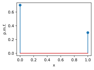

x = tf.range(-1, 2, 0.01)

def F(x):
    return 0 if x < 0 else 1 if x > 1 else 1 - p

d2l.plot(x, tf.constant([F(y) for y in x]), 'x', 'c.d.f.')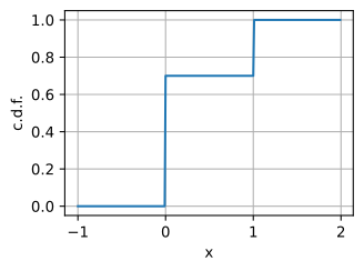

tf.cast(tf.random.uniform((10, 10)) < p, dtype=tf.float32)

<tf.Tensor: shape=(10, 10), dtype=float32, numpy=
array([[1., 1., 1., 1., 1., 0., 1., 0., 1., 0.],
       [1., 1., 1., 0., 0., 0., 0., 1., 1., 0.],
       [0., 1., 1., 0., 1., 0., 0., 1., 0., 1.],
       [0., 1., 1., 0., 0., 0., 0., 0., 0., 0.],
       [0., 0., 0., 0., 0., 0., 1., 1., 0., 0.],
       [0., 0., 0., 0., 0., 0., 0., 0., 0., 0.],
       [0., 0., 0., 1., 0., 1., 0., 0., 0., 1.],
       [0., 0., 0., 0., 1., 0., 0., 0., 0., 0.],
       [0., 1., 0., 0., 0., 0., 0., 1., 0., 0.],
       [0., 1., 0., 1., 0., 1., 0., 0., 0., 0.]], dtype=float32)>

Discrete uniform

Equally likely categories. Maximum entropy on a finite set with no prior knowledge:

n = 5

d2l.plt.stem([i+1 for i in range(n)], n*[1 / n])
d2l.plt.xlabel('x')
d2l.plt.ylabel('p.m.f.')
d2l.plt.show()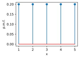

x = tf.range(-1, 6, 0.01)

def F(x):
    return 0 if x < 1 else 1 if x > n else tf.floor(x) / n

d2l.plot(x, [F(y) for y in x], 'x', 'c.d.f.')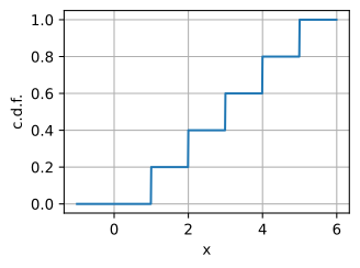

tf.random.uniform((10, 10), 1, n, dtype=tf.int32)

<tf.Tensor: shape=(10, 10), dtype=int32, numpy=
array([[2, 2, 1, 2, 4, 2, 4, 4, 1, 1],
       [2, 4, 2, 1, 2, 4, 2, 3, 1, 2],
       [4, 4, 1, 1, 4, 2, 2, 1, 3, 4],
       [2, 2, 4, 2, 2, 1, 4, 4, 1, 4],
       [4, 4, 2, 3, 4, 1, 4, 2, 1, 3],
       [4, 2, 4, 2, 2, 4, 2, 2, 1, 4],
       [1, 4, 1, 4, 2, 4, 2, 2, 4, 2],
       [1, 1, 3, 2, 1, 4, 3, 1, 3, 4],
       [4, 1, 1, 2, 1, 1, 3, 3, 1, 2],
       [4, 4, 3, 4, 4, 2, 2, 2, 3, 1]], dtype=int32)>

Continuous uniform

Density \frac{1}{b-a} on [a, b]. Source of pseudo-random samples for Monte Carlo and dropout:

a, b = 1, 3

x = tf.range(0, 4, 0.01)
p = tf.cast(x > a, tf.float32) * tf.cast(x < b, tf.float32) / (b - a)
d2l.plot(x, p, 'x', 'p.d.f.')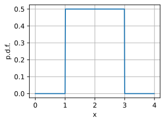

def F(x):
    return 0 if x < a else 1 if x > b else (x - a) / (b - a)

d2l.plot(x, [F(y) for y in x], 'x', 'c.d.f.')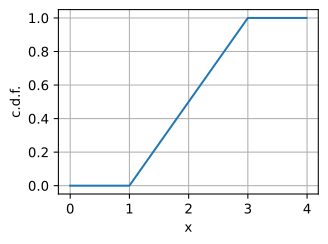

(b - a) * tf.random.uniform((10, 10)) + a

<tf.Tensor: shape=(10, 10), dtype=float32, numpy=
array([[1.7372098, 1.4449008, 2.0546732, 1.5171988, 2.4205537, 2.715879 ,
        1.6308517, 2.5322638, 2.6039743, 2.300883 ],
       [2.4029205, 2.7737122, 2.4768963, 2.8328905, 2.3471265, 2.3032713,
        2.642329 , 1.777067 , 1.9798965, 1.5024555],
       [2.0536928, 2.1130447, 1.2949264, 1.6347921, 1.1056359, 1.3375168,
...
       [2.3416533, 2.5529044, 2.4089496, 1.3706727, 1.7478693, 2.630633 ,
        2.4757807, 1.426496 , 1.8427832, 1.7212303],
       [2.0113635, 1.2461581, 1.4139686, 1.8745306, 1.1085136, 2.974681 ,
        2.8705134, 1.4228523, 1.7236967, 2.396513 ],
       [1.1791408, 1.7514703, 2.6267025, 1.9077885, 2.5822089, 1.7725577,
        1.9190166, 1.3631129, 2.7579336, 1.5572813]], dtype=float32)>

Binomial

Sum of n iid Bernoullis. Bell-shaped for large n (Gaussian limit):

n, p = 10, 0.2

# Compute binomial coefficient
def binom(n, k):
    comb = 1
    for i in range(min(k, n - k)):
        comb = comb * (n - i) // (i + 1)
    return comb

pmf = tf.constant([p**i * (1-p)**(n - i) * binom(n, i) for i in range(n + 1)])

d2l.plt.stem([i for i in range(n + 1)], pmf)
d2l.plt.xlabel('x')
d2l.plt.ylabel('p.m.f.')
d2l.plt.show()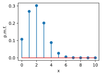

x = tf.range(-1, 11, 0.01)
cmf = tf.cumsum(pmf)

def F(x):
    return 0 if x < 0 else 1 if x > n else cmf[int(x)]

d2l.plot(x, [F(y) for y in x.numpy().tolist()], 'x', 'c.d.f.')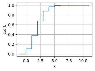

m = tfp.distributions.Binomial(n, p)
m.sample(sample_shape=(10, 10))

<tf.Tensor: shape=(10, 10), dtype=float32, numpy=
array([[8., 8., 5., 4., 5., 6., 7., 6., 5., 6.],
       [7., 8., 5., 5., 6., 4., 6., 6., 5., 5.],
       [7., 7., 5., 7., 5., 6., 7., 5., 3., 3.],
       [4., 6., 8., 6., 5., 6., 8., 2., 8., 5.],
       [7., 5., 7., 5., 5., 8., 5., 6., 6., 4.],
       [7., 7., 7., 7., 7., 5., 4., 8., 8., 5.],
       [9., 4., 6., 5., 5., 6., 5., 6., 5., 5.],
       [7., 6., 6., 6., 7., 5., 7., 8., 8., 3.],
       [7., 6., 7., 4., 6., 5., 4., 6., 6., 4.],
       [3., 3., 6., 7., 3., 7., 6., 4., 3., 6.]], dtype=float32)>

Poisson

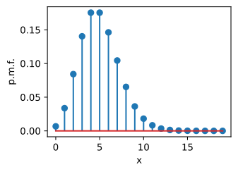
Rare events: P(X = k) = \frac{\lambda^k e^{-\lambda}}{k!}. Approximates binomial with n large, p small, np \to \lambda:

Poisson CDF

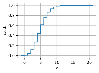
The cumulative distribution sums the probability of observing up to k events:

F(k)=P(X \le k).

Poisson samples

Sampling turns the distribution into count data: nonnegative integers with mean and variance both near \lambda.

<tf.Tensor: shape=(10, 10), dtype=float32, numpy=
array([[ 5.,  7.,  5.,  3.,  2.,  2.,  5.,  1., 10., 12.],
       [ 2.,  2.,  3.,  5., 13.,  2.,  6., 12.,  3.,  3.],
       [ 5.,  4.,  5.,  5.,  7.,  4., 10.,  3.,  8.,  8.],
       [ 4.,  6.,  5.,  4.,  4.,  5.,  5.,  4.,  8.,  2.],
       [ 2.,  7.,  7., 10.,  6.,  4.,  4.,  3.,  4.,  5.],
       [ 7.,  9.,  3.,  3.,  5.,  7.,  5.,  9.,  1.,  1.],
       [ 3.,  9.,  4.,  5.,  5.,  4.,  6.,  4.,  4.,  4.],
       [ 5.,  5.,  6.,  4.,  7.,  5.,  7.,  3.,  3.,  7.],
       [ 4.,  8.,  7.,  5.,  1.,  9.,  5.,  1.,  4.,  7.],
       [ 7.,  4.,  6.,  5.,  6.,  7.,  3.,  7.,  5.,  8.]], dtype=float32)>

Gaussian

\mathcal{N}(\mu, \sigma^2) — bell curve. CLT makes it the limit of many small contributions; that’s why it’s everywhere:

p = 0.2
ns = [1, 10, 100, 1000]
d2l.plt.figure(figsize=(10, 3))
for i in range(4):
    n = ns[i]
    pmf = tf.constant([p**i * (1-p)**(n-i) * binom(n, i)
                        for i in range(n + 1)])
    d2l.plt.subplot(1, 4, i + 1)
    d2l.plt.stem([(i - n*p)/tf.sqrt(tf.constant(n*p*(1 - p)))
                  for i in range(n + 1)], pmf)
    d2l.plt.xlim([-4, 4])
    d2l.plt.xlabel('x')
    d2l.plt.ylabel('p.m.f.')
    d2l.plt.title("n = {}".format(n))
d2l.plt.show()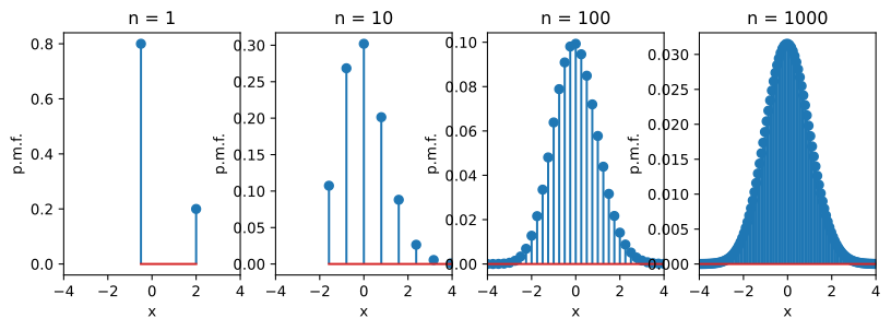

mu, sigma = 0, 1

x = tf.range(-3, 3, 0.01)
p = 1 / tf.sqrt(2 * tf.pi * sigma**2) * tf.exp(
    -(x - mu)**2 / (2 * sigma**2))

d2l.plot(x, p, 'x', 'p.d.f.')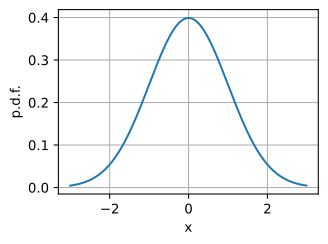

Gaussian (cont.)

Changing \mu shifts the bell curve; changing \sigma spreads it. Samples concentrate near the mean and thin out in the tails.

def phi(x):
    return (1.0 + erf((x - mu) / (sigma * tf.sqrt(tf.constant(2.))))) / 2.0

d2l.plot(x, [phi(y) for y in x.numpy().tolist()], 'x', 'c.d.f.')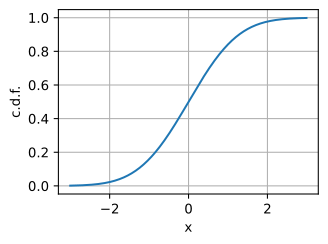

tf.random.normal((10, 10), mu, sigma)

<tf.Tensor: shape=(10, 10), dtype=float32, numpy=
array([[ 1.2940284 , -1.3513582 ,  0.43401146,  0.80263275, -1.5064023 ,
         0.5343853 ,  0.4783328 , -0.92537683,  0.21975398, -0.7574427 ],
       [-1.1687071 ,  0.7251529 ,  0.28543553,  1.1485885 ,  1.8152535 ,
        -0.38132277, -0.8599074 ,  0.8453477 , -0.33401227, -0.59957945],
       [ 0.6457711 ,  0.97372025,  0.40683332, -0.41854623, -0.4951485 ,
...
        -1.0377833 ,  1.3192103 , -0.59620786, -1.3965349 ,  0.87898743],
       [ 0.08591997, -0.38368505, -0.8918355 ,  2.4433193 ,  1.2253478 ,
        -0.09213971,  1.0231755 , -0.9645969 , -1.6856028 , -1.1013749 ],
       [ 0.15980119,  0.2718463 ,  1.1029124 ,  0.57733184,  1.9085764 ,
        -0.85503834, -0.42456862, -1.3844157 , -1.7794005 , -1.1509789 ]],
      dtype=float32)>

Recap

• A small toolkit covers most needs: Bernoulli, uniform (discrete/continuous), binomial, Poisson, Gaussian.
• CLT makes the Gaussian central — sums of many small effects look Gaussian.
• Each distribution has a closed-form NLL → standard loss in DL.