class TimeMachine(d2l.DataModule):
    """The Time Machine dataset."""
    def _download(self):
        fname = d2l.download(d2l.DATA_URL + 'timemachine.txt', self.root,
                             '090b5e7e70c295757f55df93cb0a180b9691891a')
        with open(fname) as f:
            return f.read()

data = TimeMachine()
raw_text = data._download()
raw_text[:60]From Text to Tokens
From Text to Tokens
Neural networks eat numbers; text arrives as a string. The tokenizer carves the string into the units x_t a sequence model reads, and maps each to an integer id.
- It fixes the model’s output-layer size and every document’s effective length.
- It is learned from data and ships with every modern LM: the tokenizer is part of the model.
- This section: characters/words → bytes → byte pair encoding from scratch → verified token-for-token against
tiktoken.
Read the dataset
'The Time Machine, by H. G. Wells [1898]\n\n\n\n\nI\n\n\nThe Time Tra'Classical pipelines normalized aggressively (drop punctuation, lowercase). We keep the step for the char/word experiments, but byte-level BPE will need none of it:
'the time machine by h g wells i the time traveller for so it'Characters vs. words
characters:     27 distinct,  173428 tokens in the corpus
words: 4579 distinct, 32775 tokens in the corpus- Characters: ~30 symbols, no OOV, but 170k time steps.
- Words: 5× shorter, but thousands of types, unbounded growth, and unseen words are out of vocabulary.
Vocabulary size and sequence length
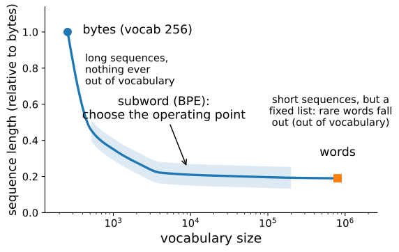
A larger vocabulary encodes the same text in fewer tokens; BPE interpolates.
Text as bytes
Every string is UTF-8 bytes: a universal base alphabet of 256 symbols. Nothing is ever out of vocabulary.
23 characters, 32 bytes
'a' -> [97]
'é' -> [195, 169]
'你' -> [228, 189, 160]
'🚀' -> [240, 159, 154, 128]
Cost: 1 byte per English character, up to 4 elsewhere. Long sequences are the price (the fertility problem, quantified later).
Byte pair encoding: merge, repeat
Count adjacent pairs, merge the most frequent into a new token, repeat. On hug pug pun bun hugs hug hug pug (32 bytes):
| step | pair | count | new token | corpus length |
|---|---|---|---|---|
| 1 | u,g |
6 | ug |
26 |
| 2 | h,ug |
4 | hug |
22 |
| 3 | hug,' ' |
3 | 'hug ' |
19 |
Greedy compression with a learned dictionary.
Merges form a tree
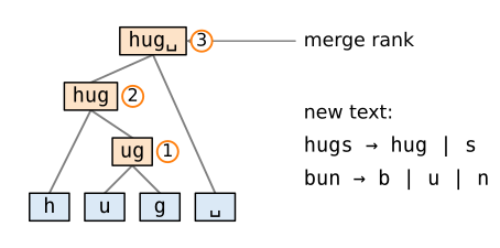
New text replays the merges: “hugs” → hug+s; rare “bun” falls back to bytes.
BPE training on a small corpus
BPETokenizer.train: ids 0–255 are bytes, each merge takes the next id, so id order = merge rank.
b'u' + b'g' -> b'ug'
b'h' + b'ug' -> b'hug'
b'hug' + b' ' -> b'hug '
Encoding = replay merges by rank
@d2l.add_to_class(BPETokenizer)
def _encode_chunk(self, text_bytes):
    ids = [self.byte_ids[b] for b in text_bytes]
    while len(ids) > 1:
        # The lowest-rank merge applicable anywhere in this chunk
        pair = min(zip(ids, ids[1:]),
                   key=lambda p: self.merges.get(p, float('inf')))
        if pair not in self.merges:
            break
        ids = self._merge(ids, pair, self.merges[pair])
    return ids

@d2l.add_to_class(BPETokenizer)
def encode(self, text, allow_special=False):
    if allow_special and self.specials:
        pat = '(' + '|'.join(regex.escape(s) for s in self.specials) + ')'
        ids = []
        for part in regex.split(pat, text):
            if part in self.specials:
                ids.append(self.specials[part])
            elif part:
                ids.extend(self.encode(part))
        return ids
    return [i for chunk in self._chunks(text)
            for i in self._encode_chunk(chunk.encode('utf-8'))]

@d2l.add_to_class(BPETokenizer)
def decode(self, ids):
    specials = {i: s.encode('utf-8') for s, i in self.specials.items()}
    data = b''.join(self.vocab[i] if i in self.vocab else specials[i]
                    for i in ids)
    return data.decode('utf-8', errors='replace')
Round trip
[b'hug', b's']
[b'b', b'u', b'n']
'hug pug hugs'
Encoding consults only the merge table: train and inference agree by construction. The merge table is the tokenizer.
Trained on The Time Machine
tok = BPETokenizer(vocab_size=1024)
tok.train(raw_text)
merged_ids = list(tok.merges.values())
print('first:', [tok.vocab[i] for i in merged_ids[:8]])
print('last: ', [tok.vocab[i] for i in merged_ids[-8:]])
ids = tok.encode('The Time Traveller smiled. Are you sure?')
print_wrapped(len(ids), 'tokens:', [tok.vocab[i] for i in ids])
first: [b'e ', b'th', b'd ', b'in', b't ', b's ', b'an', b'er']
last: [b'appe', b'vo', b'ering ', b'too ', b'door', b'acro', b'clo', b'after ']
13 tokens: [b'The ', b'Time Traveller ', b's', b'mi', b'le', b'd', b'. A',
b'r', b'e ', b'you ', b'su', b're', b'?']Compression vs. vocabulary size
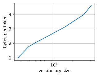
A smaller BPE vocab is a prefix of a larger one, so one training run sweeps them all:
Unconstrained merges cross word boundaries
78 tokens cross a word boundary, e.g. [', and ', 'of the ', '. I ', '. Th',
    '. A', '. I', 'in the ', 'ed to ']
Tokens like of the compress the training corpus but are brittle composites that generalize poorly.
Pre-tokenization
Split text into chunks with a regex; merges never cross chunks (GPT-2’s actual pattern):
['The',
 ' traveller',
 "'s",
 ' clock',
 ' struck',
 ' 12',
 ',',
 '345',
 ' times',
 '.']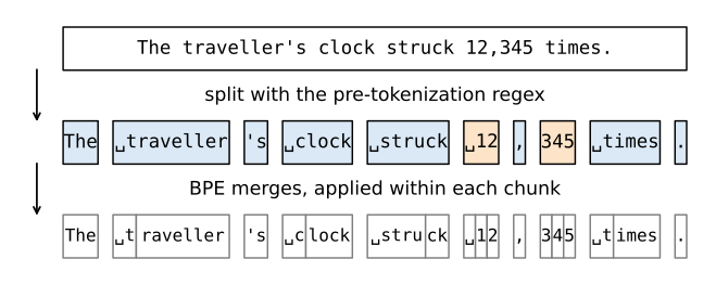
The regex first separates words, digit runs, and punctuation; BPE merges are then restricted to each resulting chunk.
Retrain with the pattern
bpe = BPETokenizer(vocab_size=1024, pattern=BPETokenizer.GPT2_PATTERN)
bpe.train(raw_text)
crossers = [v for i, v in bpe.vocab.items()
            if i >= 256 and b' ' in v.strip(b' ')]
print('boundary-crossing tokens now:', len(crossers))
gained = sorted(set(bpe.vocab.values()) - set(tok.vocab.values()),
                key=lambda v: (-len(v), v))
print_wrapped('longest tokens gained instead:',
              [v.decode('utf-8', 'replace') for v in gained[:6]])
boundary-crossing tokens now: 0
longest tokens gained instead: [' Psychologist', 'sychologist', '
Traveller', ' Morlocks', ' darkness', ' Machine']Special tokens bypass BPE
<pad>, <bos>, <eos> live above the BPE id range: they must never be producible from ordinary text (prompt-injection guard; cf. tiktoken’s allowed_special):
as plain text:   [60, 98, 111, 115, 62, 341, 513, 680]
as control code: [1025, 341, 513, 680]
pad/bos/eos ids: 1024 1025 1026 | len: 1027
What a production tokenizer stores
One table: bytes → rank, plus the pre-tokenization regex.
[(b'\xa0', 254), (b'\xad', 255), (b' t', 256), (b' a', 257), (b'he', 258), (b'in', 259)]
{'<|endoftext|>': 50256}
GPT-2’s first merges (” t”, ” a”) match what we learned from one novella: the head of English is that stable.
Comparison with the GPT-2 tokenizer
Load GPT-2’s published ranks into our encoder and reproduce tiktoken token for token:
ours = BPETokenizer.from_tiktoken('gpt2')
para = ('The Time Traveller (for so it will be convenient to speak of '
        'him) was expounding a recondite matter to us; his pale grey '
        'eyes shone and twinkled. Prices rose 3.5% in 1895, and naïve '
        'café patrons paid £12,345 more! 🚀')
assert ours.encode(para) == enc.encode(para)
print(len(ours.encode(para)), 'tokens, identical to tiktoken')
print([ours.vocab[i].decode('utf-8', 'replace')
       for i in ours.encode(para)[:8]])
60 tokens, identical to tiktoken
['The', ' Time', ' Trave', 'ller', ' (', 'for', ' so', ' it']Fertility across languages
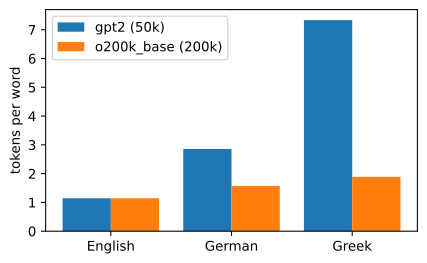
Same sentence: ~1 token/word in English, ~7 in Greek under GPT-2; o200k_base narrows the gap to ~2.
Digits and glitch tokens
gpt2: 12345678 -> ['123', '45', '678']
o200k_base: 12345678 -> ['123', '456', '78']- Token boundaries misalign with place value → brittle arithmetic.
- Glitch tokens (” SolidGoldMagikarp”): frequent in the tokenizer’s corpus, absent from the model’s, leaving an untrained embedding reachable from any prompt.
Recap
- Chars ↔︎ words is a vocabulary/length trade-off; bytes make the base alphabet universal.
- BPE: iterated most-frequent-pair merges; encoding replays merges by rank; the merge table is the tokenizer.
- Pre-tokenization keeps merges inside words; specials live outside the BPE range.
- Production tokenizers are exactly this at scale, and we reproduced GPT-2’s tokenization token for token.