%matplotlib inline
from d2l import torch as d2l
import torch
from torch import nnTwo autoregressive strategies
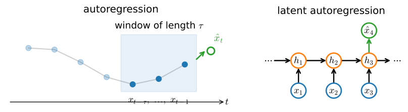
A fixed window discards observations beyond lag \tau; a recurrent state keeps fixed memory while updating a learned function of the entire prefix.
Fixed window = the n-gram (and, later, an attention context window). Latent state = the RNN and the state space models of the next chapters.
Generating data
A noisy sine wave, 1000 time steps:
class Data(d2l.DataModule):
    def __init__(self, batch_size=16, T=1000, num_train=600, tau=4):
        self.save_hyperparameters()
        self.time = d2l.arange(1, T + 1, dtype=d2l.float32)
        self.x = d2l.sin(0.01 * self.time) + d2l.randn(T) * 0.2
data = Data()
d2l.plot(data.time, data.x, 'time', 'x', xlim=[1, 1000], figsize=(6, 3))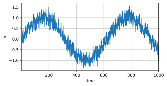
Autoregressive features
Each example predicts x_t from the last \tau values, \mathbf{x}_t = (x_{t-\tau}, \ldots, x_{t-1}). Fit a linear model on the first 600 windows:
def get_dataloader(self, train):
    features = [self.x[i : self.T-self.tau+i] for i in range(self.tau)]
    self.features = d2l.stack(features, 1)
    self.labels = d2l.reshape(self.x[self.tau:], (-1, 1))
    i = slice(0, self.num_train) if train else slice(self.num_train, None)
    return self.get_tensorloader([self.features, self.labels], train, i)
model = d2l.LinearRegression(lr=0.01)
trainer = d2l.Trainer(max_epochs=5)
trainer.fit(model, data)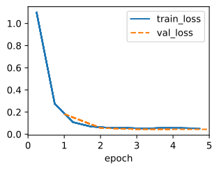
One-step prediction
Predict \hat{x}_t from the true previous \tau values. Tracks the series closely:
onestep_preds = d2l.numpy(model(data.features))
d2l.plot(data.time[data.tau:], [data.labels, onestep_preds], 'time', 'x',
         legend=['labels', '1-step preds'], figsize=(6, 3))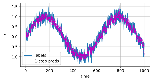
Multistep rollout
Forecasting many steps ahead means feeding predicted values back as inputs, so errors compound:
multistep_preds = d2l.zeros(data.T)
multistep_preds[:] = data.x
for i in range(data.num_train + data.tau, data.T):
    multistep_preds[i] = model(
        d2l.reshape(multistep_preds[i-data.tau : i], (1, -1)))
multistep_preds = d2l.numpy(multistep_preds)
d2l.plot([data.time[data.tau:], data.time[data.num_train+data.tau:]],
[onestep_preds, multistep_preds[data.num_train+data.tau:]], 'time',
'x', legend=['1-step preds', 'multistep preds'], figsize=(6, 3))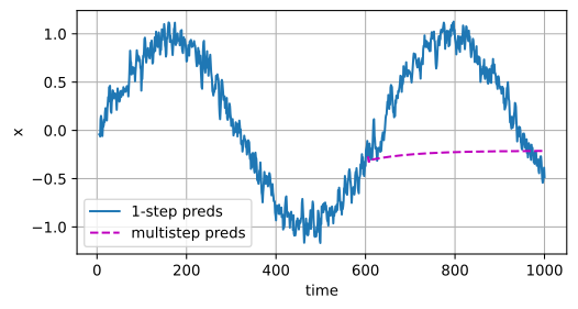
def k_step_pred(k):
    features = []
    for i in range(data.tau):
        features.append(data.x[i : i+data.T-data.tau-k+1])
    # The (i+tau)-th element stores the (i+1)-step-ahead predictions
    for i in range(k):
        preds = model(d2l.stack(features[i : i+data.tau], 1))
        features.append(d2l.reshape(preds, -1))
    return features[data.tau:]
steps = (1, 4, 16, 64)
preds = k_step_pred(steps[-1])
d2l.plot(data.time[data.tau+steps[-1]-1:],
[d2l.numpy(preds[k-1]) for k in steps], 'time', 'x',
legend=[f'{k}-step preds' for k in steps], figsize=(6, 3))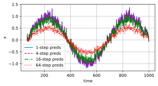
1- and 4-step curves track the truth; longer horizons are increasingly damped, and a full rollout collapses to a near-constant. Long-horizon forecasting is hard.