from d2l import torch as d2l
import torchRecurrent Neural Networks
Recurrent Neural Networks
A recurrent neural network carries a hidden state \mathbf{h}_t across time steps, a learned summary of all input seen so far:
\mathbf{h}_t = \phi(\mathbf{W}_{xh}\mathbf{x}_t + \mathbf{W}_{hh}\mathbf{h}_{t-1} + \mathbf{b}).
Same weights at every step, so the parameter count is constant regardless of sequence length. Unbounded effective context (in principle), with no fixed-size window like an n-gram.
Unrolled in time
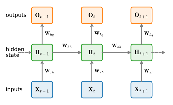
An RNN unrolled across three time steps; the same weights are reused at every step.
Setup
The recurrence in code
The naive form: two matrix multiplies, summed:
tensor([[-0.5367, -0.1777,  2.4283, -0.5488],
        [ 5.6435, -1.8725,  2.6781,  0.3557],
        [ 3.8535, -1.2030,  3.6370, -1.0466]])
Equivalently, concatenate input and hidden and multiply by the concatenated weight matrix. Same result, one matmul:
tensor([[-0.5367, -0.1777,  2.4283, -0.5488],
        [ 5.6435, -1.8725,  2.6781,  0.3557],
        [ 3.8535, -1.2030,  3.6370, -1.0466]])
The concatenate-then-multiply form is what most framework RNN implementations actually do.
Constant memory per step
- \mathbf{h}_t has a fixed size, independent of t.
- To form \mathbf{h}_t we need only \mathbf{h}_{t-1} and \mathbf{x}_t; everything older can be dropped.
- Any-length input at flat per-step memory and compute.
- The trade: the state is a lossy summary, so it must learn what to keep. Attention (later) keeps everything instead, at a cost that grows with length.
As a language model
- Embedding maps a BPE token id to a vector \mathbf{x}_t.
- RNN updates the hidden state \mathbf{h}_t.
- Linear head projects \mathbf{h}_t to vocab logits; softmax gives P(x_{t+1} \mid x_{\le t}).
- Loss = cross-entropy with the next-token target.
Teacher forcing
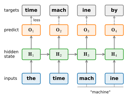
Targets are the inputs shifted forward by one token; each step predicts the next token.
Train on gold prefixes; generate on the model’s own outputs. That mismatch is the rollout-error problem again.
Recap
- RNN: \mathbf{h}_t = \phi(\mathbf{W}_{xh}\mathbf{x}_t + \mathbf{W}_{hh}\mathbf{h}_{t-1} + \mathbf{b}).
- Same parameters at every step; the hidden state is a fixed-size summary of the whole past.
- Trains by backprop through time: gradients flow from \mathbf{h}_T back to every earlier hidden state.
- Those long products vanish or explode on long sequences, fixed by LSTM and GRU in the next chapter.