Gated RNNs fixed the memory problem and kept a compute problem: \mathbf{H}_t needs \mathbf{H}_{t-1}, so training is sequential in t while GPUs sit idle. CNNs (ch. 6) compute all positions at once.
Goal: parallel training, O(1)-state inference. Two passes at it:
Strip the GRU until its state update is linear → evaluate the whole sequence with a parallel scan (minGRU).
Rebuild properly from continuous time → state space models: principled gates (\Delta), stability by construction, recurrence \equiv convolution, HiPPO memory, S4D.
Substitute it into itself: \mathbf{H}_{t-2} is buried under two nested \phi’s. Nonlinear compositions don’t simplify: the nonlinearity on the state path creates the sequential dependency.
Input-derived gates, nonlinear readouts, and depth between layers do not prevent a scan. Removing \mathbf{H}_{t-1} from the nonlinearities is the required change.
minGRU: two cuts
From the GRU: gates and candidate from the input only (the reset gate then has nothing to reset, so it is deleted):
Now affine in the state: \mathbf{H}_t = \mathbf{a}_t \odot \mathbf{H}_{t-1} + \mathbf{b}_t with \mathbf{a}_t = 1 - \mathbf{Z}_t, \mathbf{b}_t = \mathbf{Z}_t \odot \tilde{\mathbf{H}}_t with all coefficients computable for all t at once.
Memory is readable: input from k steps back is scaled by \prod_j \mathbf{a}_j \in (0,1): eigenvalues in plain sight (8.6).
The parallel scan
Represent step t by the affine map (\mathbf{a}_t, \mathbf{b}_t). Composition is again affine, and associative:
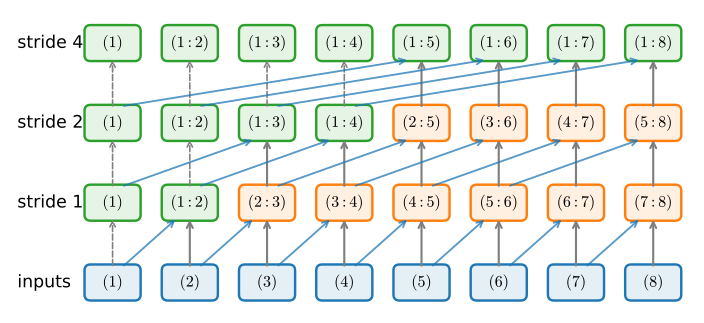
Any associative “running total” parallelizes (Blelloch, 1990):
Doubling strides 1, 2, 4: after \log_2 T rounds every position holds its prefix.
Implementation
One round per stride; each round is a batched multiply-add:
def associative_scan(a, b, dim=0):"""Parallel prefix scan for h_t = a_t * h_{t-1} + b_t with h_0 = 0.""" a, b = a.movedim(dim, 0), b.movedim(dim, 0) step =1while step < b.shape[0]: # ceil(log2 T) rounds of combines a_prev, b_prev = a[:-step], b[:-step] a, b = (torch.cat([a[:step], a_prev * a[step:]]), torch.cat([b[:step], a[step:] * b_prev + b[step:]])) step *=2return b.movedim(0, dim)
def sequential_scan(a, b): h, outputs = d2l.zeros_like(b[0]), []for t inrange(b.shape[0]): h = a[t] * h + b[t] outputs.append(h)return d2l.stack(outputs, 0)a, b = torch.rand(100, 4, 8), torch.randn(100, 4, 8)err = (associative_scan(a, b) - sequential_scan(a, b)).abs().max()print(f'maximum deviation: {float(err):.2e}')
maximum deviation: 4.77e-07
Trains like a CNN
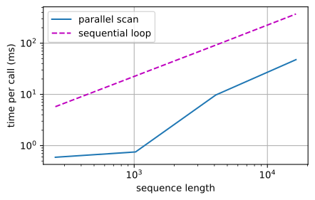
Scan vs. sequential loop, batch 32, 128 units:
device = d2l.try_gpu()def wall_clock(f, *args, reps=3): f(*args) # Warm upif device.type=='cuda': torch.cuda.synchronize() start = time.time()for _ inrange(reps): f(*args)if device.type=='cuda': torch.cuda.synchronize()return (time.time() - start) / repslengths, times = [256, 1024, 4096, 16384], [[], []]for T in lengths: a = torch.rand(T, 32, 128, device=device) b = torch.randn(T, 32, 128, device=device) times[0].append(wall_clock(associative_scan, a, b) *1e3) times[1].append(wall_clock(sequential_scan, a, b) *1e3)d2l.plot(lengths, times, 'sequence length', 'time per call (ms)', legend=['parallel scan', 'sequential loop'], xscale='log', yscale='log', figsize=(5, 3))
The loop grows linearly in T; the scan’s few rounds saturate the GPU. Inference is unchanged: still one token, one state update at a time.
A minGRU cell
Drop-in replacement for the gated cells of the previous section, with no time loop; a carried state folds into \mathbf{b}_1:
class MinGRU(d2l.Module):"""The minimal GRU: input-only gates and a linear state path."""def__init__(self, num_inputs, num_hiddens):super().__init__()self.save_hyperparameters()self.W_xz = nn.Linear(num_inputs, num_hiddens)self.W_xh = nn.Linear(num_inputs, num_hiddens)def forward(self, inputs, H=None): Z = torch.sigmoid(self.W_xz(inputs)) # (num_steps, batch, hiddens) H_tilde = torch.tanh(self.W_xh(inputs)) a, b =1- Z, Z * H_tildeif H isnotNone: # Fold the carried-in state into the first step b = torch.cat([b[:1] + a[:1] * H, b[1:]]) outputs = associative_scan(a, b)return outputs, outputs[-1]
Language modeling, same recipe as the LSTM’s
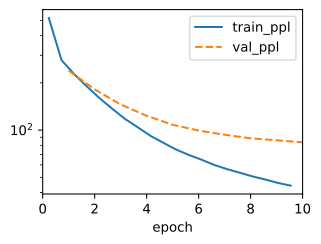
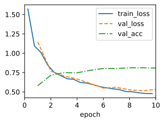
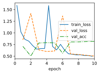
Time Machine, 1,024-token BPE, 50k windows of 32, emb 64, hidden 128, 10 epochs, clip 1:
data = d2l.TimeMachine(batch_size=1024, num_steps=32,
                       num_train=50000, num_val=5000)
Why continuous? It parameterizes a law of motion, not a table of step weights: one extra scalar \Delta (step size) converts (\mathbf{A},
\mathbf{B}) into a recurrence at any sampling rate.
\Delta \to 0: \bar{\mathbf{A}} \to \mathbf{I}, \bar{\mathbf{B}} \to 0. Copy the state, ignore the input.
\Delta large: \bar{\mathbf{A}} \to 0. Overwrite from the input.
A learned \Deltais an update gate, not bolted on: it fell out of the calculus. (Next section: \Delta becomes input-dependent.)
Identity in the worked scalar mode a=-1: backward Euler gives x_t = (1-z)x_{t-1} + z u_t with z = \sigma(\log \Delta): the GRU gate is a discretization rule there (Gu, 2023).
Menu of rules: ZOH / bilinear (S4’s choice) / backward Euler all keep stability at any \Delta; forward Euler does not. In code: expm1.
Stability by construction: store a_n = -e^{\theta_n}, then |\bar{a}_n| = e^{\Delta\,\mathrm{Re}(a_n)} < 1 for every parameter value; diagonal (normal) \mathbf{A} ⇒ no transients either. No clipping, no knife-edge (8.6).
Recurrence is convolution
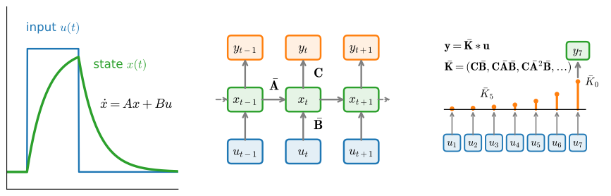
LTI: the same \bar{\mathbf{A}}, \bar{\mathbf{B}}, \mathbf{C} at every step. Unroll:
One model, three views: ODE, recurrence, convolution.
Three views, one answer
num_states, num_steps, delta =8, 64, 0.1a =-torch.arange(1., num_states +1) # Re(a) < 0b, c = torch.ones(num_states), torch.randn(num_states)a_bar = torch.exp(delta * a) # Zero-order holdb_bar = torch.expm1(delta * a) / a * b # expm1: accurate e^x - 1u = torch.randn(num_steps)x, ys = torch.zeros(num_states), [] # (i) recurrencefor t inrange(num_steps): x = a_bar * x + b_bar * u[t] ys.append(torch.dot(c, x))y_loop = torch.stack(ys)xs = associative_scan(a_bar.tile(num_steps, 1), # (ii) parallel scan b_bar * u[:, None])y_scan = xs @ ck = torch.arange(num_steps)[:, None] # (iii) convolutionkernel = (c * b_bar * a_bar ** k).sum(-1)y_conv = torch.tensor(np.convolve(u, kernel)[:num_steps])print(f'scan vs loop: {float((y_scan - y_loop).abs().max()):.2e}, 'f'conv vs loop: {float((y_conv - y_loop).abs().max()):.2e}')
scan vs loop: 2.38e-07, conv vs loop: 2.38e-07
S4 trains through the conv view with FFTs (O(T \log T)); we keep the scan, because it survives the input-dependent dynamics of the next section; the kernel view will not.
What should A be? HiPPO
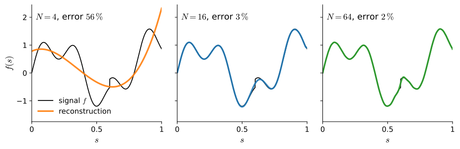
The state is N numbers summarizing all history. Which N lose least? HiPPO: make \mathbf{x}(t) the coefficients of the optimal polynomial approximation of the past; maintaining it online is a linear, time-varying ODE with a fixed matrix pattern: \dot{\mathbf{x}} = (\mathbf{A}\mathbf{x} + \mathbf{B}u)/t (A_{nn} = -(n{+}1), B_n = \sqrt{2n+1}) — the 1/t tracks the uniform measure over a growing past.
Reconstructing 1,000 steps of history from the final state alone.
Three objects: online LegS projection (owns the theorem) → S4 = LTI model initialized at the HiPPO matrix (DPLR kernels, solved Long Range Arena) → S4D = diagonal approximation (matches S4 empirically; init a_n = -(n{+}1) is multiscale, not optimal). Plus S5: the scan. We implement S4D’s parameterization with S5’s scan.
The S4D layer
Per channel: N-state diagonal SSM; learnable \log \Delta per channel (log-uniform init: gates of many speeds); \mathbf{B} = \mathbf{1}; three lines of ZOH + the scan:
class S4D(nn.Module):"""A diagonal state space layer: one SSM per feature channel."""def__init__(self, num_hiddens, num_states=4, dt_min=0.001, dt_max=0.1):super().__init__() H, N = num_hiddens, num_statesself.log_a = nn.Parameter( torch.log(torch.arange(1., N +1)).repeat(H, 1))self.log_dt = nn.Parameter( torch.rand(H, 1) * math.log(dt_max / dt_min) + math.log(dt_min))self.C = nn.Parameter(torch.randn(H, N) / math.sqrt(N))self.D = nn.Parameter(torch.ones(H))def forward(self, u): # (num_steps, batch, num_hiddens) a =-torch.exp(self.log_a) # (H, N), Re(a) < 0 da = torch.exp(self.log_dt) * a a_bar = torch.exp(da) b_bar = torch.expm1(da) / a # ZOH with B = 1 a_elems = a_bar.expand(u.shape[0], 1, -1, -1) # Same at every step b_elems = b_bar * u.unsqueeze(-1) # (T, batch, H, N) x = associative_scan(a_elems, b_elems)return (x *self.C).sum(-1) +self.D * u
The S4D block
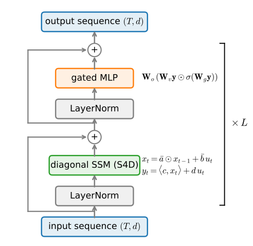
SSM mixes time, gated MLP mixes channels and restores nonlinearity:
class S4DBlock(nn.Module):def__init__(self, num_hiddens, num_states):super().__init__()self.ln1 = nn.LayerNorm(num_hiddens)self.ssm = S4D(num_hiddens, num_states)self.ln2 = nn.LayerNorm(num_hiddens)self.W_v = nn.Linear(num_hiddens, 2* num_hiddens)self.W_g = nn.Linear(num_hiddens, 2* num_hiddens)self.W_o = nn.Linear(2* num_hiddens, num_hiddens)def forward(self, X): X = X +self.ssm(self.ln1(X)) Y =self.ln2(X)return X +self.W_o(self.W_v(Y) * torch.sigmoid(self.W_g(Y)))
Sequential Fashion-MNIST
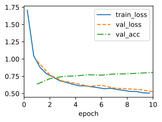
784 pixels, one at a time. The readout decides the question: mean-pool all outputs = mixing benchmark; read the final step only = retention diagnostic. Same head, data, epochs, clip 1 (the LSTM destabilizes without it; the S4D can’t explode); S4D stack vs. parameter-matched LSTM (~30k params each):
data = d2l.FashionMNIST(batch_size=128)results = {}def train_and_report(name, model, epochs=10): trainer = d2l.Trainer(max_epochs=epochs, gradient_clip_val=1, num_gpus=1) start = time.time() trainer.fit(model, data) params =sum(p.numel() for p in model.parameters() if p.requires_grad) results[name] = (params, float(model.board.data['val_acc'][-1].y), (time.time() - start) / epochs)s4d = SeqClassifier(nn.Sequential(*[S4DBlock(48, 4) for _ inrange(2)]), num_hiddens=48)train_and_report('S4D', s4d)
print(f'{"model":>12}{"params":>8}{"val acc":>8}{"s/epoch":>8}')for name, (params, acc, secs) in results.items():print(f'{name:>12}{params:>8,}{acc:>8.3f}{secs:>8.1f}')
       model   params  val acc  s/epoch
         S4D   30,058    0.808     47.6
 S4D (final)   30,058    0.806     36.9
        LSTM   29,930    0.819      4.0
S4D (mean-pool): low-to-mid 80s in both frameworks, every rerun. S4D (final state): within run-to-run noise of it — the memory really is in the state after 784 steps, not rescued by early outputs.
LSTM: 60-84% across reruns, tracking init defaults: plain uniform init leaves memory to chance, orthogonal weights improve the odds, and parity takes the full folklore (+ forget bias 1).
The \Delta-init hands the S4D multi-scale memory by design; the LSTM gets it only from initialization folklore.
On Long Range Arena tasks of up to 16k steps, this family first surpassed the compared baselines.
Inference, one token at a time
Training used the scan; the bargain’s other half is recurrent inference. Nothing to derive: the discretized update is the algorithm. State: one (H, N) block per layer; the gated MLP is position-wise and carries none.
@d2l.add_to_class(S4D)def step(self, u, x=None):"""Advance one token: u is (batch, H); x is the (batch, H, N) state.""" a =-torch.exp(self.log_a) da = torch.exp(self.log_dt) * a a_bar = torch.exp(da) # Same ZOH as forward b_bar = torch.expm1(da) / aif x isNone: x = u.new_zeros(*u.shape, a_bar.shape[-1]) x = a_bar * x + b_bar * u.unsqueeze(-1) # One recurrence stepreturn (x *self.C).sum(-1) +self.D * u, x@d2l.add_to_class(S4DBlock)def step(self, X, x=None):"""Advance the block one token; only the SSM carries state.""" y, x =self.ssm.step(self.ln1(X), x) X = X + y Y =self.ln2(X)return X +self.W_o(self.W_v(Y) * torch.sigmoid(self.W_g(Y))), x
Stepped == scanned, on the trained model
Replay validation images through the trained encoder both ways: all 784 pixels by scan, then one at a time by step:
X_val =next(iter(data.val_dataloader()))[0][:64].to(d2l.try_gpu())with torch.no_grad(): seq = s4d.emb(X_val.reshape(X_val.shape[0], -1, 1).movedim(1, 0)) y_scan = s4d.encoder(seq) # All 784 steps at once states, ys = [None] *len(s4d.encoder), []for t inrange(seq.shape[0]): # One pixel at a time X, new_states = seq[t], []for blk, x inzip(s4d.encoder, states): X, x = blk.step(X, x) new_states.append(x) states, ys = new_states, ys + [X]err =float((torch.stack(ys) - y_scan).abs().max())scale =float(y_scan.abs().max())print(f'stepped vs scanned: deviation {err:.2e} 'f'on activations of scale {scale:.0f}: relative {err / scale:.2e}')assert err <1e-3* scale
stepped vs scanned: deviation 4.41e-04 on activations of scale 71: relative 6.21e-06
Same arithmetic, different association order: float-level agreement. The assert doubles as a regression guard.
Recurrent Decoding Has Constant Persistent State
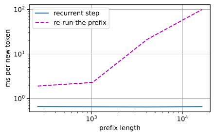
Cost of absorbing the next token after a prefix of P, batch of 32 streams:
def one_step(X, states):with torch.no_grad():for i, blk inenumerate(s4d.encoder): X, states[i] = blk.step(X, states[i])return Xdef rerun(seq):with torch.no_grad():return s4d.encoder(seq)lengths, times = [256, 1024, 4096, 16384], [[], []]states = [None] *len(s4d.encoder)for P in lengths: seq = torch.randn(P, 32, 48, device=device) one_step(seq[-1], states) # Materialize the state times[0].append(wall_clock(one_step, seq[-1], states) *1e3) times[1].append(wall_clock(rerun, seq) *1e3)d2l.plot(lengths, times, 'prefix length', 'ms per new token', legend=['recurrent step', 're-run the prefix'], xscale='log', yscale='log', figsize=(5, 3))print(f'carried state: {sum(4* x.numel() for x in states) //32} 'f'bytes per sequence, at every prefix length')
carried state: 1536 bytes per sequence, at every prefix length
Re-running the prefix grows with P; the step is flat.
Entire memory: ~1.5 KiB of state per sequence, at any length: vs. a KV cache that grows tens of KiB per token (ch. on transformers).
Recap
Linear state path → affine maps → associative scan: O(\log T) depth training, O(1)-state inference.
minGRU ≈ GRU quality on our LM recipe.
SSMs: \Deltais a gate; eigenvalues inside the unit circle by construction; recurrence \equiv convolution \equiv ODE.
HiPPO: a fixed-size state provably carries a long past — via a time-varying system; frozen, its matrix initializes S4/S4D.
Inference delivered: step == scan to float precision; flat cost per token; ~1 KiB of state vs. a KV cache that grows with context.
The update remains LTI: the kernel is fixed before the model sees the data, so the state update is content-blind (the MLPs around it are not). Fixing that (and keeping the scan) is the next section.