def matrix_state_dual(Q, K, V, a):
    """Y = (L o Q K^T) V with L_ts = a_t ... a_{s+1} for t >= s, else 0."""
    cum = torch.cumsum(torch.log(a), 0)
    logL = cum[:, None] - cum[None, :]                  # Sum of logs over (s, t]
    causal = torch.tril(torch.ones(len(a), len(a), dtype=torch.bool,
                                   device=a.device))
    L = torch.exp(logL.masked_fill(~causal, -torch.inf))
    return (L * (Q @ K.T)) @ V

err = (matrix_state_dual(Q, K, V, a) - y_rec).abs().max() / y_rec.abs().max()
print(f'relative deviation, dual vs recurrence: {float(err):.2e}')
assert err < 1e-3                          # Two orders, one computation

ones = torch.ones(T, device=device)                     # All a_t = 1
err = (matrix_state_dual(Q, K, V, ones)
       - torch.tril(Q @ K.T) @ V).abs().max()
print(f'a_t = 1, deviation from masked linear attention: {float(err):.2e}')
assert err < 1e-6 # L is literally the causal maskMatrix-State Recurrences and State Space Duality
Dive into Deep Learning · §12.4
The matrix state
one recurrence · measured capacity · transition structure · state-space duality · chunked training · model families
The Matrix-State Recurrence
Ch. 10 ended linear attention as a recurrence; ch. 12 built selective SSMs from continuous time. Same object:
\mathbf{S}_t = \mathbf{D}_t\, \mathbf{S}_{t-1} + \mathbf{k}_t \mathbf{v}_t^\top, \qquad \mathbf{o}_t = \mathbf{S}_t^\top \mathbf{q}_t
- The transition \mathbf{D}_t determines retained state; the outer product \mathbf{k}_t\mathbf{v}_t^\top writes new state.
- Linear attention: \mathbf{D}_t = \mathbf{I} — never forget.
What the modern family drops from ch. 10’s construction: the feature map \phi and the normalizer state \mathbf{z} (output normalization instead). The mLSTM retains \mathbf{z}.
Measured Memory Cost
Store n unit-norm pairs, read key j: \mathbf{S}^\top \mathbf{k}_j = \mathbf{v}_j + \sum_{i \neq j} (\mathbf{k}_i^\top \mathbf{k}_j)\,\mathbf{v}_i
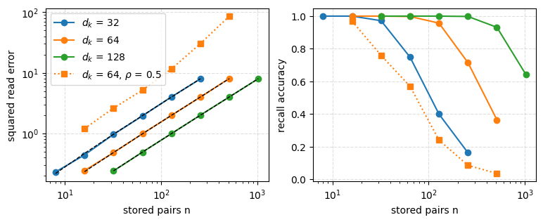
- Measured error on the (n-1)/d_k prediction — for i.i.d. isotropic unit keys; recall collapses past n \approx d_k.
- Correlated keys (dotted) revive the cancelled cross terms: width stops helping.
- Capacity is set by width, not time: interference comes from other stored pairs.
Forms of Decay
Three one-line fixes for crowding, on the same recurrence:
\gamma\,\mathbf{S}_{t-1} \;\to\; a_t\,\mathbf{S}_{t-1} \;\to\; \mathrm{diag}(\boldsymbol{\alpha}_t)\,\mathbf{S}_{t-1}\;\; (+\;\mathbf{k}_t\mathbf{v}_t^\top)
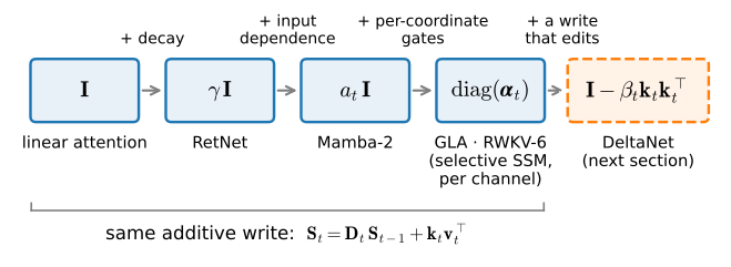
- RetNet: fixed \gamma per head · Mamba-2: input-dependent scalar · GLA / RWKV-6: input-dependent diagonal — the selective SSM per channel.
Unroll it: the state-space duality
\mathbf{Y} = \big(\mathbf{L} \circ \mathbf{Q}\mathbf{K}^\top\big)\,\mathbf{V}, \qquad L_{ts} = a_t\, a_{t-1} \cdots a_{s+1}
The pivot: all a_t = 1 → \mathbf{L} is the causal mask. A gated linear recurrence is attention with a learned, decaying mask (SSD, Dao & Gu 2024).
- Quadratic mode: materialize \mathbf{L} \circ \mathbf{Q}\mathbf{K}^\top — attention.
- Linear mode: sweep the sum left to right — the recurrence, state \mathbf{S}_t.
- Two contraction orders, one computation — an identity for this scalar-gated (1-semiseparable) linear family, not softmax attention.
The duality, asserted
relative deviation, dual vs recurrence: 5.11e-06
a_t = 1, deviation from masked linear attention: 0.00e+00- Agreement to float rounding; at a_t = 1 the dual reduces exactly to ch. 10’s masked linear attention.
- This computation verifies the recurrent form of masked linear attention introduced in Chapter 10.
Chunked: mostly matmul, a little scan
Partition the semiseparable matrix into chunks of C tokens:
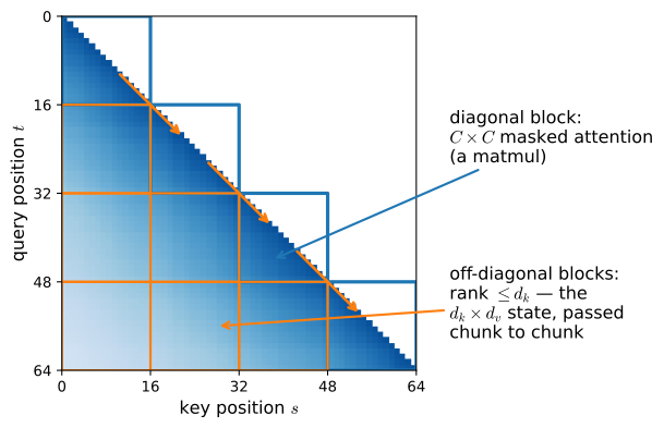
- Diagonal blocks: C \times C masked-attention matmuls, all parallel.
- Off-diagonal blocks: rank \le d_k — a d_k \times d_v state passed chunk to chunk, T/C steps.
A dozen lines, verified
segsum builds the within-chunk mask in log space (-\infty above the diagonal, before any exponential):
def segsum(log_a):
    """Segment sums: (..., C) -> (..., C, C) with entries sum over (s, t]."""
    C = log_a.shape[-1]
    cum = torch.cumsum(log_a, -1)
    diff = cum[..., :, None] - cum[..., None, :]
    keep = torch.tril(torch.ones(C, C, dtype=torch.bool, device=log_a.device))
    return diff.masked_fill(~keep, -torch.inf)          # Mask in log space

def matrix_state_chunked(Q, K, V, a, chunk_size=64):
    """The same Y, chunk by chunk: attention inside, recurrence across."""
    T, C = Q.shape[0], chunk_size
    Qc, Kc = Q.view(-1, C, Q.shape[-1]), K.view(-1, C, K.shape[-1])
    Vc, log_a = V.view(-1, C, V.shape[-1]), torch.log(a).view(-1, C)
    L = torch.exp(segsum(log_a))                        # (T/C, C, C)
    b = torch.exp(torch.cumsum(log_a, -1))              # Decay since chunk entry
    Y = (L * (Qc @ Kc.transpose(-1, -2))) @ Vc          # Diagonal blocks
    S = Q.new_zeros(Q.shape[-1], V.shape[-1])
    for c in range(T // C):                             # T/C boundary steps
        Y[c] += (Qc[c] * b[c][:, None]) @ S             # Read the carried state
        S = b[c][-1] * S + (Kc[c] * (b[c][-1] / b[c])[:, None]).T @ Vc[c]
    return Y.reshape(T, -1)

for chunk_size in [16, 64, 256]:
    err = ((matrix_state_chunked(Q, K, V, a, chunk_size) - y_rec).abs().max()
           / y_rec.abs().max())
    print(f'chunk size {chunk_size:4d}: relative deviation {float(err):.2e}')
    assert err < 1e-3                      # Chunked == recurrence
chunk size 16: relative deviation 1.92e-07
chunk size 64: relative deviation 6.81e-07
chunk size 256: relative deviation 1.75e-06Measured Time–Memory Tradeoff
C interpolates recurrence (C = 1) → quadratic dual (C = T):
           form  time (ms)  peak (MiB)
     recurrence     282.93         3.0
   chunked (16)      36.12         1.5
   chunked (64)       9.42         3.0
  chunked (256)       2.61        12.0
 chunked (1024)       0.87        48.0
 quadratic dual       1.01       272.0
(NVIDIA GeForce RTX 4090, float32, torch 2.11.0+cu128; teaching implementations, warmed up)- Token loop: launch-bound, slowest by far. Dual: matmul-fast, T^2 memory.
- Chunked: matmul speed at an order of magnitude less memory.
Measured Hardware Performance
- Tensor cores run matmuls; Mamba-1’s scan is elementwise (bandwidth-bound). Mamba-2’s scalar transition buys the chunked form.
- The paper’s empirical scaling observation: training several times faster and state size N: 16 → 64–256 at little extra wall clock — the capacity law says what that buys.
- Frontier: Mamba-3 upgrades the discretization itself (trapezoidal rule, complex states, MIMO).
per layer, per sequence, fp16:
matrix state, one 64x64 head:      0.01 MiB, constant
Mamba-2 2.7B, SSM 655,360 + conv 15,360 elements: 1.28 MiB, constant
GQA KV cache at n =     4,096:    16.00 MiB and growing
GQA KV cache at n =   131,072:   512.00 MiB and growing
GQA KV cache at n = 1,048,576:  4096.00 MiB and growing
The flat line vs. the growing cache — the hybrid-design problem of the chapter’s last section.
Model Family
| model | transition \mathbf{D}_t | write |
|---|---|---|
| linear attention | \mathbf{I} | add \phi(\mathbf{k}_t)\mathbf{v}_t^\top |
| RetNet | \gamma\,\mathbf{I} fixed | add \mathbf{k}_t\mathbf{v}_t^\top |
| Mamba | input-dep. diagonal (per channel) | add \Delta_t u_t \mathbf{B}_t |
| GLA / RWKV-6 | input-dep. diagonal | add \mathbf{k}_t\mathbf{v}_t^\top |
| Mamba-2 | input-dep. scalar | add \mathbf{k}_t\mathbf{v}_t^\top |
| mLSTM | scalar exp-gates + normalizer | add i_t\,\mathbf{k}_t\mathbf{v}_t^\top |
Three lineages — attention, SSMs, RNNs — one recurrence. Read the write column: every row only adds.
mLSTM: the one that kept the normalizer
\mathbf{S}_t = f_t \mathbf{S}_{t-1} + i_t \mathbf{k}_t\mathbf{v}_t^\top, \quad \mathbf{z}_t = f_t \mathbf{z}_{t-1} + i_t \mathbf{k}_t, \quad \mathbf{o}_t = \frac{\mathbf{S}_t^\top \mathbf{q}_t}{\max(|\mathbf{z}_t^\top \mathbf{q}_t|, 1)}
Exponential gates i_t = \exp(\tilde{i}_t) overflow float32 in a few dozen steps; the fix is online softmax’s running max, carried as a state m_t.
torch.manual_seed(0)
d_k, d_v, T = 8, 8, 64
q, k, v = (torch.randn(T, d) for d in (d_k, d_k, d_v))
i_pre, f_pre = torch.randn(T), 2.0 + torch.randn(T)  # Gate pre-activations

def mlstm_naive(q, k, v, i_pre, f_pre, dtype):
    """The unstabilized recurrence, in a given precision."""
    q, k, v = q.to(dtype), k.to(dtype), v.to(dtype)
    i_g, f_g = i_pre.to(dtype).exp(), f_pre.to(dtype).exp()
    S, z = torch.zeros(d_k, d_v, dtype=dtype), torch.zeros(d_k, dtype=dtype)
    outputs = []
    for t in range(T):
        S = f_g[t] * S + i_g[t] * (k[t][:, None] * v[t][None, :])
        z = f_g[t] * z + i_g[t] * k[t]
        outputs.append(q[t] @ S / (q[t] @ z).abs().clamp(min=1))
    return torch.stack(outputs)

def mlstm_stabilized(q, k, v, i_pre, f_pre):
    """Carry m_t and rescale the past, as in online softmax."""
    S, z = torch.zeros(d_k, d_v), torch.zeros(d_k)
    m = torch.tensor(-torch.inf)
    outputs = []
    for t in range(T):
        m_new = torch.maximum(f_pre[t] + m, i_pre[t])
        f_g, i_g = torch.exp(f_pre[t] + m - m_new), torch.exp(i_pre[t] - m_new)
        S = f_g * S + i_g * (k[t][:, None] * v[t][None, :])
        z = f_g * z + i_g * k[t]
        m = m_new
        outputs.append(q[t] @ S
                       / torch.maximum((q[t] @ z).abs(), torch.exp(-m)))
    return torch.stack(outputs)

exact = mlstm_naive(q, k, v, i_pre, f_pre, torch.float64)
naive = mlstm_naive(q, k, v, i_pre, f_pre, torch.float32)
bad = ~torch.isfinite(naive).all(-1)        # argmax(bool) would report 0
first_bad = int(bad.float().argmax()) if bool(bad.any()) else 'none'
stab = mlstm_stabilized(q, k, v, i_pre, f_pre)
err = (stab - exact.float()).abs().max() / exact.abs().max()
print(f'float32 unstabilized: first non-finite output at step {first_bad}')
print(f'float32 stabilized vs float64: relative deviation {float(err):.2e}')
assert torch.isfinite(stab).all() and err < 1e-3
float32 unstabilized: first non-finite output at step 49
float32 stabilized vs float64: relative deviation 2.02e-05Limitations of Additive Writes
- Decay manages crowding; it does not cure it — forgetting is indiscriminate, interference is specific.
- Not one model in the table can edit what it wrote about \mathbf{k} without decaying everything else.
The fast weight programmers’ repair (1990s → 2021): read what the memory holds at \mathbf{k}_t, write only the correction.
The next section introduces DeltaNet, whose corrective write can edit an existing binding.