Gated Recurrence

BPTT’s verdict: the gradient k steps back scales as \rho^k: vanishing or exploding. Clipping fixes explosion; vanishing needs architecture.

The fix that stuck: multiplicative gating (Hochreiter & Schmidhuber, 1997).

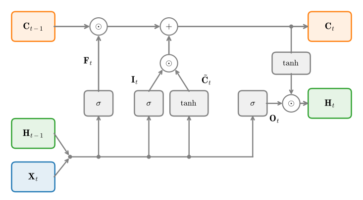
LSTM: a protected memory cell + three learned gates.
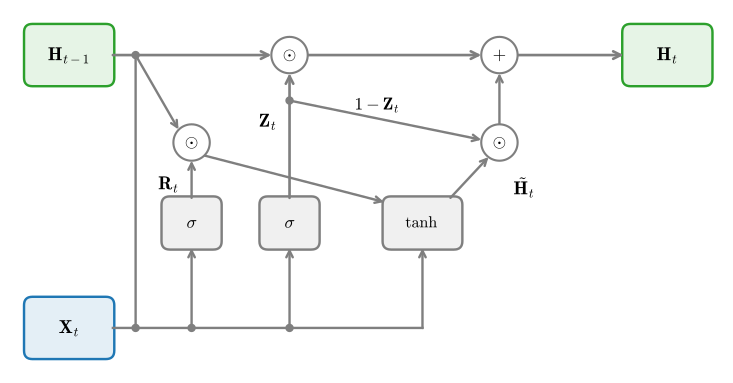
GRU: the streamlined two-gate version.
Depth and direction, compressed to their surviving lessons.
The same gate primitive lives on in SwiGLU MLPs, Mamba, xLSTM — and in every linear recurrence of this chapter.

The gate

The only recurrence whose Jacobian is exactly the identity is an accumulator: \mathbf{S}_t = \mathbf{S}_{t-1} + (\textrm{new}). But it never forgets. Memory needs decisions: write? clear? reveal?

Make the decision differentiable:

\mathbf{G}_t = \sigma(\mathbf{X}_t \mathbf{W}_{xg} + \mathbf{H}_{t-1} \mathbf{W}_{hg} + \mathbf{b}_g) \in (0,1)^h,

used as an elementwise multiplier: 1 = pass, 0 = block.

Learned, context-dependent, per unit and per step.
Along the gated path a perturbation scales by \prod_j g_{j}\leq 1: no explosion, and g \approx 1 preserves memory losslessly.

The LSTM memory cell

The cell state is touched only by an elementwise product and a sum; gates control write, keep, and reveal.

LSTM equations

Three sigmoid gates plus a \tanh input node, same algebra four times:

\mathbf{I}_t, \mathbf{F}_t, \mathbf{O}_t = \sigma(\mathbf{X}_t \mathbf{W}_{x\cdot} + \mathbf{H}_{t-1} \mathbf{W}_{h\cdot} + \mathbf{b}),\quad \tilde{\mathbf{C}}_t = \tanh(\cdots).

The update that matters:

\mathbf{C}_t = \mathbf{F}_t \odot \mathbf{C}_{t-1} + \mathbf{I}_t \odot \tilde{\mathbf{C}}_t,\qquad \mathbf{H}_t = \mathbf{O}_t \odot \tanh(\mathbf{C}_t).

Direct path (gates held fixed): \partial \mathbf{C}_t/\partial \mathbf{C}_{t-1} = \textrm{diag}(\mathbf{F}_t): hold \mathbf{F} \approx 1, \mathbf{I} \approx 0 and the cell (and its gradient) survives: the constant error carousel.
The total derivative adds gate paths through \mathbf{H}_{t-1}: an additive route is supplied, not a guarantee.
\mathbf{O}_t lets a cell accumulate silently, then reveal.

From scratch: parameters

Four heads, one triple() factory each; num_inputs is the embedding dimension:

class LSTMScratch(d2l.Module):
    """The long short-term memory (LSTM) cell implemented from scratch."""
    def __init__(self, num_inputs, num_hiddens, sigma=0.01):
        super().__init__()
        self.save_hyperparameters()

        init_weight = lambda *shape: nn.Parameter(d2l.randn(*shape) * sigma)
        triple = lambda: (init_weight(num_inputs, num_hiddens),
                          init_weight(num_hiddens, num_hiddens),
                          nn.Parameter(d2l.zeros(num_hiddens)))
        self.W_xi, self.W_hi, self.b_i = triple()  # Input gate
        self.W_xf, self.W_hf, self.b_f = triple()  # Forget gate
        self.W_xo, self.W_ho, self.b_o = triple()  # Output gate
        self.W_xc, self.W_hc, self.b_c = triple()  # Input node

Forward pass

Walk the sequence, carry (\mathbf{H}, \mathbf{C}):

@d2l.add_to_class(LSTMScratch)
def forward(self, inputs, H_C=None):
    if H_C is None:
        # Initial state with shape: (batch_size, num_hiddens)
        H = d2l.zeros((inputs.shape[1], self.num_hiddens),
                      device=inputs.device)
        C = d2l.zeros((inputs.shape[1], self.num_hiddens),
                      device=inputs.device)
    else:
        H, C = H_C
    outputs = []
    for X in inputs:
        I = d2l.sigmoid(d2l.matmul(X, self.W_xi) +
                        d2l.matmul(H, self.W_hi) + self.b_i)
        F = d2l.sigmoid(d2l.matmul(X, self.W_xf) +
                        d2l.matmul(H, self.W_hf) + self.b_f)
        O = d2l.sigmoid(d2l.matmul(X, self.W_xo) +
                        d2l.matmul(H, self.W_ho) + self.b_o)
        C_tilde = d2l.tanh(d2l.matmul(X, self.W_xc) +
                           d2l.matmul(H, self.W_hc) + self.b_c)
        C = F * C + I * C_tilde
        H = O * d2l.tanh(C)
        outputs.append(H)
    return outputs, (H, C)

lstm = LSTMScratch(num_inputs=16, num_hiddens=32)
X = d2l.ones((9, 4, 16))  # (num_steps, batch_size, num_inputs)
outputs, (H, C) = lstm(X)
d2l.check_shape(outputs[-1], (4, 32))
d2l.check_shape(H, (4, 32))
d2l.check_shape(C, (4, 32))

Training on The Time Machine

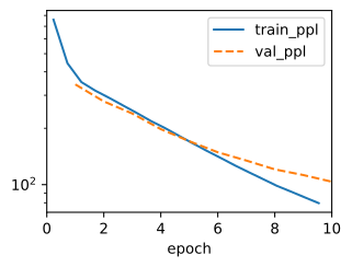
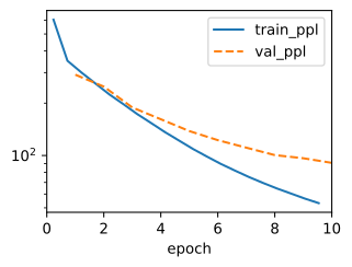
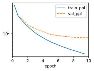
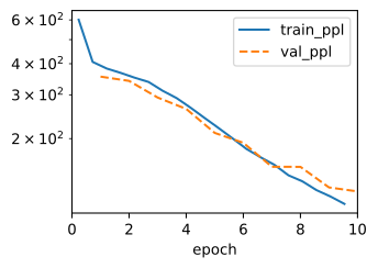
Same recipe as the vanilla RNN (50k windows of 32 BPE tokens, batch 1024, emb 64, hidden 128, 10 epochs, clip 1), so the numbers are directly comparable:

data = d2l.TimeMachine(batch_size=1024, num_steps=32,
                       num_train=50000, num_val=5000)

lstm = LSTMScratch(num_inputs=64, num_hiddens=128)
model = d2l.RNNLMScratch(lstm, vocab_size=len(data.vocab), lr=4)

trainer = d2l.Trainer(max_epochs=10, gradient_clip_val=1, num_gpus=1)
model.board.yscale = 'log'
trainer.fit(model, data)

Reading the result

def val_ppl(model):
    return float(model.board.data['val_ppl'][-1].y)

ppls = {'LSTM (scratch)': val_ppl(model)}
print(f"validation perplexity {ppls['LSTM (scratch)']:.1f}")

validation perplexity 103.7

Vanilla RNN under the identical recipe: val ppl ~90–110. The scratch LSTM only matches it. Why:

10 epochs is short for 4h(d{+}h{+}1) recurrent weights (vs. h(d{+}h{+}1)); the curves are still moving.
Naive init leaves every gate half-open: \sigma(0)=0.5 halves the cell each step until the biases move. Fix: \mathbf{b}_f = 1 (exercise).

Concise: the fused layer

Eight matmuls per step make the fused kernel matter even more than for the vanilla RNN. Same interface, plus num_layers:

class LSTM(d2l.RNN):
    """The multilayer LSTM model implemented with high-level APIs."""
    def __init__(self, num_inputs, num_hiddens, num_layers=1, dropout=0):
        d2l.Module.__init__(self)
        self.save_hyperparameters()
        self.rnn = nn.LSTM(num_inputs, num_hiddens, num_layers,
                           dropout=dropout)

    def forward(self, inputs, H_C=None):
        return self.rnn(inputs, H_C)

Train and generate

lstm = LSTM(num_inputs=64, num_hiddens=128)
model = d2l.RNNLM(lstm, vocab_size=len(data.vocab), lr=4)

trainer = d2l.Trainer(max_epochs=10, gradient_clip_val=1, num_gpus=1)
model.board.yscale = 'log'
trainer.fit(model, data)

ppls['LSTM'] = val_ppl(model)
pred = model.predict('the time traveller', 30, data.tokenizer, d2l.try_gpu(),
                     temperature=0.5)
print(f"perplexity {ppls['LSTM']:.1f}, {pred!r}")

perplexity 90.7, "the time travellering, and\npresently\ntism.\n\n'I had a viola, and\ntowing\ns"

GRU: two gates, no cell

Cho et al. (2014): drop the separate cell state, merge to two gates.

\tilde{\mathbf{H}}_t = \tanh(\mathbf{X}_t \mathbf{W}_{xh} + (\mathbf{R}_t \odot \mathbf{H}_{t-1}) \mathbf{W}_{hh} + \mathbf{b}_h), \mathbf{H}_t = \mathbf{Z}_t \odot \mathbf{H}_{t-1} + (1 - \mathbf{Z}_t) \odot \tilde{\mathbf{H}}_t.

Reset gates the past inside the candidate; update convex-blends old and new.

GRU in code

class GRU(d2l.RNN):
    """The multilayer GRU model implemented with high-level APIs."""
    def __init__(self, num_inputs, num_hiddens, num_layers=1, dropout=0):
        d2l.Module.__init__(self)
        self.save_hyperparameters()
        self.rnn = nn.GRU(num_inputs, num_hiddens, num_layers,
                          dropout=dropout)

gru = GRU(num_inputs=64, num_hiddens=128)
model = d2l.RNNLM(gru, vocab_size=len(data.vocab), lr=4)

trainer = d2l.Trainer(max_epochs=10, gradient_clip_val=1, num_gpus=1)
model.board.yscale = 'log'
trainer.fit(model, data)

ppls['GRU'] = val_ppl(model)
print(f"validation perplexity {ppls['GRU']:.1f}")

validation perplexity 79.2

Three quarters of the LSTM’s recurrent parameters and the best perplexity in this section’s runs: fewer gates converge faster on a short budget. Its 2020s legacy: strip the gates to input-only functions and the recurrence turns linear → minGRU, LRU, SSMs.

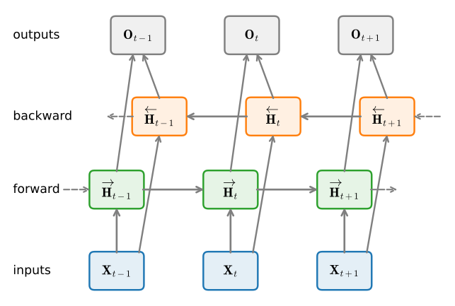
Depth and direction, briefly

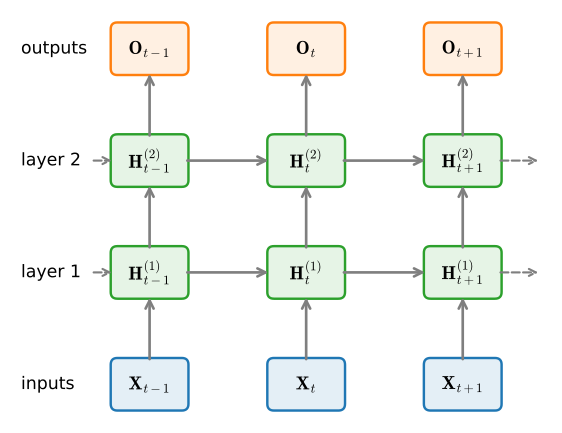
Layer l reads layer l{-}1 at the same step and itself at the previous step; a one-argument change with num_layers:

Two stacked recurrent layers over three time steps.

lstm2 = LSTM(num_inputs=64, num_hiddens=128, num_layers=2)
model = d2l.RNNLM(lstm2, vocab_size=len(data.vocab), lr=4)
trainer = d2l.Trainer(max_epochs=10, gradient_clip_val=1, num_gpus=1)
model.board.yscale = 'log'
trainer.fit(model, data)

ppls['LSTM (2 layers)'] = val_ppl(model)
print(f'{"model":>16} {"val ppl":>8}')
for name, p in ppls.items():
    print(f'{name:>16} {p:>8.1f}')

           model  val ppl
  LSTM (scratch)    103.7
            LSTM     90.7
             GRU     79.2
 LSTM (2 layers)    122.7

Read the scoreboard: the second layer does not pay on a corpus this small. Depth pays at scale; knowing when it won’t is craft.

Bidirectional RNNs

Two chains, one forward and one backward, concatenated per step, so every output conditions on the whole sequence:

Forward + backward chains, outputs read 2h features.

birnn = nn.LSTM(64, 128, bidirectional=True)
X = d2l.randn(32, 8, 64)  # (num_steps, batch_size, num_inputs)
outputs, (H, C) = birnn(X)
outputs.shape, H.shape

(torch.Size([32, 8, 256]), torch.Size([2, 8, 128]))

No use unchanged as a causal decoder: at sampling time the future does not exist; “next-token training” hands the model the answer. Use for tagging/encoding (ELMo → BERT); fine inside generative systems as the encoder.

Gates everywhere

Where	The gate	Controls
LSTM	forget \mathbf{F}_t	cell-state decay
GRU	update \mathbf{Z}_t	copy vs. overwrite
Highway nets	transform gate	depth routing
GLU/SwiGLU MLPs	\sigma/Swish branch	channel selection
Mamba	step size \Delta_t	linear-state decay
Griffin / mLSTM	recurrence gates	linear-cell decay

SwiGLU’s payoff: measured in the transformer chapter’s matched-parameter sweep.
xLSTM: exponential gates (log-space stabilized) revive the classic cell; its matrix sibling mLSTM joins the family table two sections ahead.
Bottom rows: gates from the input only → linear recurrence → parallel training. The rest of the chapter rides that step.

Recap

Vanishing gradients are architectural; the cure is an additive state path plus learned multiplicative gates.
LSTM: \mathbf{C}_t = \mathbf{F}_t \odot \mathbf{C}_{t-1} + \mathbf{I}_t \odot \tilde{\mathbf{C}}_t is the constant error carousel (the protected direct path).
GRU: two gates, convex blend, cheaper, and the section’s best perplexity: it beats the vanilla RNN clearly.
The LSTM needs budget and init care before its machinery pays: architecture and optimization are judged together.
Depth = stacked cells (rarely paid); bidirectional = encoder-only.
The gate outlived the RNN: SwiGLU, Mamba’s \Delta_t, xLSTM — input-only gates open the door to linear recurrence, next.