Practice

Dive into Deep Learning · §9.12

The craft of training
the disclosed recipe · clipping · weight averaging · how to tune

The recipe, as disclosed

What frontier runs report shipping — practice, not gospel

run	optimizer	\beta_1,\beta_2	peak LR, schedule	warmup	clip	wd
Llama 3 405B	AdamW	—	8{\times}10^{-5}, cosine	8k	—	—
DeepSeek-V3	AdamW	0.9, 0.95	2.2{\times}10^{-4}, WSD-like	2k	1.0	0.1
OLMo 2 7B	AdamW	0.9, 0.95	3{\times}10^{-4}, cosine	2k	1.0	0.1*
Kimi K2	MuonClip	—	2{\times}10^{-4}, WSD	500	—	0.1

• Consensus core: AdamW (0.9, 0.95) · wd 0.1 with exemptions · clip 1.0 · warmup + cosine-or-WSD · early batch ramp.
• Blanks are data too: the recipe travels as code defaults, not prose.
• One break in the optimizer column: K2 runs the Muon split (§9.9) inside an otherwise consensus recipe.

Gradient clipping in three lines

Global norm, all parameters as one vector:

\mathbf{g} \leftarrow \min\left(1,\; \frac{\theta}{\|\mathbf{g}\|_2}\right) \mathbf{g}

Direction kept, length capped. Met in ch. 8 for RNNs — it outlived the architecture: every disclosed threshold in the table is 1.

class Clipped:
    """Clip the global gradient norm before every optimizer step."""
    def __init__(self, optimizer, params, max_norm=1.0):
        self.optimizer = optimizer
        self.params = list(params)
        self.max_norm = max_norm
        self.norms = []

    def step(self):
        norm = nn.utils.clip_grad_norm_(self.params, self.max_norm)
        self.norms.append(float(norm))
        self.optimizer.step()

    def zero_grad(self):
        self.optimizer.zero_grad()

A NaN, averted

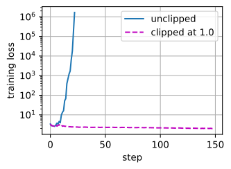
§9.6’s knife edge: SGD’s best lr sat one grid point below a NaN. Rerun the divergent point, with and without the guard:

• Unclipped: oversized step → steeper ground → bigger gradient → momentum compounds → overflow.
• Clipped, same lr: trains to the tuned run’s range.

Six steps out of two thousand

The instrumented run: median gradient norm ~0.3, threshold 1.0 — clipping changed the update on 6 of 2,000 steps.

• A fuse, not a brake: language-model gradient noise is heavy-tailed (Zhang et al., 2020); the guard exists for the tail.
• Firing on most steps = a learning-rate cut in disguise. Lower \eta or raise \theta.
• Adam: steps sit near \eta in steady state (transients up to ~3×), so clipping is no substitute for lowering a too-large \eta — it guards \mathbf{m}, \mathbf{v} from one huge gradient lingering 1/(1-\beta_2) steps.

The stability kit at scale

Clipping is one item. The rest aims at attention logits and the softmax:

• z-loss (PaLM): penalize \log^2 Z of the softmax normalizer.
• QK-norm (OLMo 2): normalize q, k right before their dot product.
• QK-clip (MuonClip): cap the largest attention logit — 15.5T tokens, zero spikes (§9.9).

When prevention fails: PaLM rewound ~100 steps and skipped the batches — same data replayed later caused no spike; state and data conspire. The OPT logbook: two months of restarts and lr cuts, published as-is.

Weight averaging

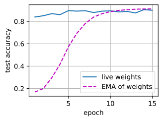
Third decision, third tool: quench noise without touching the rate — \bar{\mathbf{x}}_t = \alpha \bar{\mathbf{x}}_{t-1} + (1-\alpha)\mathbf{x}_t, the chapter’s leaky average, now on the weights (SWA; Izmailov et al., 2018).

• Window must fill first — the early gap is lag on stale iterates, not a bias to correct; warm up the decay or start late.
• Then: modestly above the live weights, and no when-to-stop lottery.

Averaging: where it matters

• Constant rate + EMA ≈ decayed schedule: decay and averaging quench the same noise (§9.8’s schedule-free view). On an already-decayed run this size: too small to call from a single run.
• LLMs: checkpoint averaging (LAWA); Llama 3 shipped an average of its annealing checkpoints. Model soups: average fine-tuned models.
• Diffusion (ch. 15): EMA is mandatory — quality tracks the window so tightly that Karras et al. (2024) reconstruct the EMA post hoc to tune it.

How to tune

The Tuning Playbook’s vocabulary

• Scientific hyperparameters: the question. Nuisance: re-tune per arm, or the comparison is void. Fixed: the claim’s fine print.
• This chapter, named: optimizer scientific, lr nuisance (four-point grid per contestant), all else fixed and stated.
• Schmidt et al. (2021): several optimizers at defaults ≈ one optimizer heavily tuned. Untuned comparisons measure effort, not algorithms.

Budgets: few runs → consensus recipe, sweep peak lr only. Tens → add wd + schedule (\eta\lambda is a ridge, §9.7). And log everything: config, seed, the one change, the NaNs. The log is the experiment.

What we did not teach, and where it lives

• SAM: flat minima at 2× gradient cost — wins concentrate in vision and fine-tuning.
• Variance reduction: beautiful finite-sum theory, never paid off for deep nets → ch. 25.
• LARS/LAMB: superseded — re-tuned momentum/AdamW match them at the same batch sizes.
• Systems: sharding state, data parallelism, overlap → ch. 11 and the training-systems appendix.

Recap: three decisions

• Direction: a norm — gradient, sign, or orthogonalized (§9.2, §9.6, §9.9).
• Step size over time: warmup, cosine, WSD (§9.8) — plus clip 1.0 as the fuse.
• Noise: batch (§9.4, §9.10), momentum (§9.5), averaging (here).

The recipe table is one coordinated setting of all three. When a run misbehaves, ask which decision is failing. Optimizers change; the decomposition has been stable for decades.