%matplotlib inline
from d2l import torch as d2l
import numpy as np
import time
import torch
from torch import nn

A = torch.zeros(256, 256)
B = torch.randn(256, 256)
C = torch.randn(256, 256)Full-batch and single-example updates
b = 1500: one well-aimed update per epoch — stalls after ~6 steps:
def train_sgd(lr, batch_size, num_epochs=2):
    data_iter, feature_dim = get_data_ch11(batch_size)
    return train_ch11(
        sgd, None, {'lr': lr}, data_iter, feature_dim, num_epochs)

gd_res = train_sgd(0.9, 1500, 10)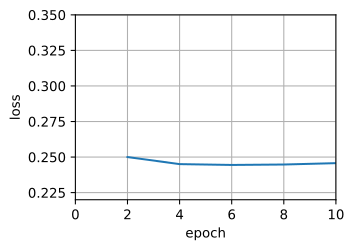
loss: 0.242, 0.016 sec/epochb = 1: 1500 updates per epoch, but 1500 tiny dispatches — more clock time per epoch than GD:
sgd_res = train_sgd(0.005, 1)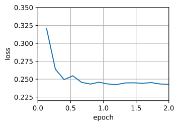
loss: 0.243, 0.401 sec/epochMinibatch timing comparison
mini1_res = train_sgd(.4, 100)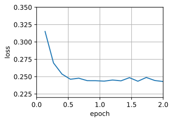
loss: 0.247, 0.016 sec/epochmini2_res = train_sgd(.05, 10)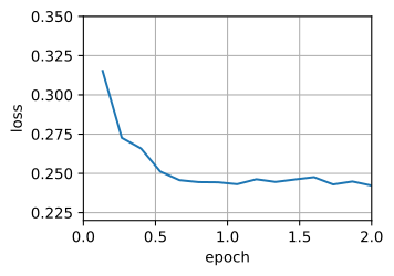
loss: 0.247, 0.055 sec/epochd2l.set_figsize([6, 3])
d2l.plot(*list(map(list, zip(gd_res, sgd_res, mini1_res, mini2_res))),
'time (sec)', 'loss', xlim=[1e-2, 10], xscale='log',
legend=['gd', 'sgd', 'batch size=100', 'batch size=10'])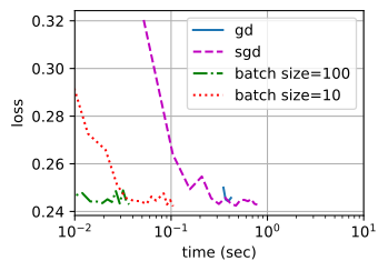
On the elapsed-time axis, b=100 reaches a given loss sooner than either extreme.
Concise: framework optimizer
The built-in optimizer runs through the same harness used later in the chapter:
def train_concise_ch11(trainer_fn, hyperparams, data_iter, num_epochs=4):
    # Initialization
    net = nn.Sequential(nn.Linear(5, 1))
    def init_weights(module):
        if type(module) == nn.Linear:
            torch.nn.init.normal_(module.weight, std=0.01)
    net.apply(init_weights)

    optimizer = trainer_fn(net.parameters(), **hyperparams)
    loss = nn.MSELoss(reduction='none')
    animator = d2l.Animator(xlabel='epoch', ylabel='loss',
                            xlim=[0, num_epochs], ylim=[0.22, 0.35])
    n, timer = 0, d2l.Timer()
    for _ in range(num_epochs):
        for X, y in data_iter:
            optimizer.zero_grad()
            out = net(X)
            y = y.reshape(out.shape)
            l = loss(out, y)
            l.mean().backward()
            optimizer.step()
            n += X.shape[0]
            if n % 200 == 0:
                timer.stop()
                # `MSELoss` computes squared error without the 1/2 factor
                animator.add(n/X.shape[0]/len(data_iter),
                             (d2l.evaluate_loss(net, data_iter, loss) / 2,))
                timer.start()
    print(f'loss: {animator.Y[0][-1]:.3f}, {timer.sum()/num_epochs:.3f} sec/epoch')
data_iter, _ = get_data_ch11(10)
trainer = torch.optim.SGD
train_concise_ch11(trainer, {'lr': 0.01}, data_iter)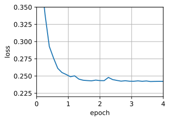
loss: 0.243, 0.058 sec/epoch