Batch Size

Dive into Deep Learning · §9.10

How large a batch?
the gradient-noise scale · steps to a target · learning-rate rules · batch ramps

Two reasons to batch, one open question

Motivation

  • §9.3, statistics: gradient variance \propto 1/b.
  • §9.4, mechanics: a batch amortizes dispatch and keeps the device fed.
  • Neither says when to stop. A bigger batch costs proportionally more compute per step — when does it stop buying an equal cut in steps?

The answer is a property of the optimization problem, not the hardware — and it changes as training proceeds.

The gradient-noise scale

A minibatch gradient is signal + noise: squared length \|\nabla f\|^2 plus \operatorname{tr}\boldsymbol{\Sigma}/b. They trade places at

b_{\textrm{noise}} = \frac{\operatorname{tr} \boldsymbol{\Sigma}}{\|\nabla f\|^2}

(McCandlish et al., 2018).

  • b \ll b_{\textrm{noise}}: mostly noise — doubling b removes half of what obscures the descent direction.
  • b \gg b_{\textrm{noise}}: essentially exact — more averaging polishes digits the update never uses.

Measure it with two batch sizes

Take expectations of the squared norm:

\mathbb{E}\big[\|\hat{\mathbf{g}}_b\|^2\big] = \|\nabla f\|^2 + \frac{\operatorname{tr} \boldsymbol{\Sigma}}{b}.

A minibatch gradient is longer than the true one — by exactly the noise power. Two batch sizes → two equations → both unknowns:

def grad_sq_norm(model, X, Y):
    logits = model(X)
    loss = F.cross_entropy(logits.reshape(-1, logits.shape[-1]),
                           Y.reshape(-1))
    grads = torch.autograd.grad(loss, list(model.parameters()))
    return sum((g ** 2).sum() for g in grads)

def noise_scale(model, X, Y, b_small=16, b_big=2048, m=400):
    def mean_sq_norm(b, m):
        idx = torch.randint(0, len(Y), (m, b), device=X.device)
        return torch.stack([grad_sq_norm(model, X[i], Y[i])
                            for i in idx]).mean()
    n_small, n_big = mean_sq_norm(b_small, m), mean_sq_norm(b_big, m // 8)
    tr_sigma = (n_small - n_big) / (1 / b_small - 1 / b_big)
    sq_norm = (b_big * n_big - b_small * n_small) / (b_big - b_small)
    return (tr_sigma / sq_norm).item()

The noise scale grows during training

CNN, then TinyLM — at initialization and after 500 steps of Adam:

noise scale at initialization: 98
after 500 steps of Adam: 705
noise scale at initialization: 2.5
after 500 steps of Adam: 113
  • Tens of examples (CNN) and single-digit sequence counts (TinyLM) at init; severalfold to two orders of magnitude larger 500 steps later.

For large language models, measured noise scales run to the millions of tokens (McCandlish et al., 2018). The magnitude does not transfer; the growth does.

Steps to a target: the prediction

Train to a fixed loss at many batch sizes; count steps S and examples E = bS. The noisy-quadratic model gives one hyperbola:

\frac{S(b)}{S_{\min}} = 1 + \frac{b_{\textrm{noise}}}{b}, \qquad \frac{E(b)}{E_{\min}} = 1 + \frac{b}{b_{\textrm{noise}}}.

  • Below b_{\textrm{noise}}: perfect scaling — double b, halve S, E constant.
  • Above: S floors at S_{\min}, examples wasted.
  • Elbow (both at 2\times their minimum) = critical batch size.

Protocol

Fixed target loss on a fixed evaluation batch, checked every 10 steps (per-minibatch training loss would bias the small-batch runs). Adam; \eta tuned at one anchor b_0, moved by the \sqrt{b/b_0} rule. Single seeded runs, read qualitatively.

def eval_loss(model, X, Y, chunk=4096):
    with torch.no_grad():
        losses = []
        for i in range(0, len(Y), chunk):
            logits = model(X[i:i + chunk])
            losses.append(F.cross_entropy(
                logits.reshape(-1, logits.shape[-1]),
                Y[i:i + chunk].reshape(-1)))
    return torch.stack(losses).mean().item()

def train_to_target(model, data, optimizer, X_eval, Y_eval, target,
                    max_steps, eval_every=10):
    model.to(device)
    step = 0
    while step < max_steps:
        for X, Y in data.train_dataloader():
            X, Y = X.to(device), Y.to(device)
            logits = model(X)
            loss = F.cross_entropy(logits.reshape(-1, logits.shape[-1]),
                                   Y.reshape(-1))
            optimizer.zero_grad()
            loss.backward()
            optimizer.step()
            step += 1
            if step % eval_every == 0 and \
               eval_loss(model, X_eval, Y_eval) <= target:
                return step
            if step >= max_steps:
                break
    return float('inf')

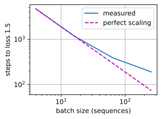
TinyLM: steps to loss 1.5

b=   4  steps=  4720  examples=   18880
b=  16  steps=  1180  examples=   18880
b=  64  steps=   390  examples=   24960
b= 256  steps=   190  examples=   48640
  • b=4 \to 16 tracks perfect scaling; examples barely move.
  • By b=256 the curve has left the line: a quadrupled batch buys about half the steps or less, and examples-to-target climbs.
  • Elbow within a small factor of the mid-training noise scale.

Same experiment, CNN
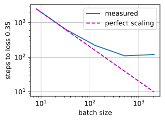
b=   8  steps=  2510  examples=   20080
b=  32  steps=   640  examples=   20480
b= 128  steps=   220  examples=   28160
b= 512  steps=   110  examples=   56320
b=2048  steps=   120  examples=  245760

At the top of the range a quadrupled batch — quadrupled compute per step — cuts the step count by at most a third, and in some runs the count rises; examples-to-target sits several times above its minimum.

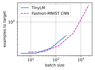
The bill in examples

  • Flat while batching is free; bends upward past the critical batch size.
  • A menu, not a verdict: height = compute, leftward = fewer steps = time.
  • Below the elbow, parallelism is free speed. Above it, halving the steps costs a doubling of the compute.

Moving the learning rate with the batch

\eta(b) = \frac{b}{b_0}\, \eta_0 \;\;\textrm{(SGD)}, \qquad \eta(b) = \sqrt{\frac{b}{b_0}}\, \eta_0 \;\;\textrm{(adaptive)}.

  • Linear: the noise floor depends on \eta/b only — hold it fixed (Goyal et al., 2017). Small-b limit of \eta_{\textrm{opt}}(b) = \eta_{\max}/(1 + b_{\textrm{noise}}/b): the rule expires at the noise scale.
  • Square root: Adam’s preconditioner already divides by the gradient’s RMS; the full SDE rule also moves \beta_i and \epsilon, and reduces to \eta \propto \sqrt{b} when they barely move (Malladi et al., 2022).

Verification: the basin slides

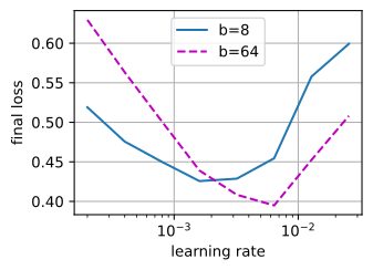
Loss vs. \eta at b=8 and b=64, fixed example budget:
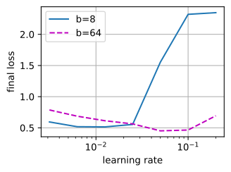
b=  8  lr=0.003125  loss=0.594
b=  8  lr=0.00625  loss=0.518
b=  8  lr=0.0125  loss=0.515
b=  8  lr=0.025  loss=0.554
b=  8  lr=0.05  loss=1.554
b=  8  lr=0.1  loss=2.321
...
b= 64  lr=0.00625  loss=0.687
b= 64  lr=0.0125  loss=0.614
b= 64  lr=0.025  loss=0.563
b= 64  lr=0.05  loss=0.451
b= 64  lr=0.1  loss=0.465
b= 64  lr=0.2  loss=0.693
b=  8  lr=0.0002  loss=0.519
b=  8  lr=0.0004  loss=0.476
b=  8  lr=0.0008  loss=0.450
b=  8  lr=0.0016  loss=0.426
b=  8  lr=0.0032  loss=0.429
b=  8  lr=0.0064  loss=0.455
...
b= 64  lr=0.0008  loss=0.501
b= 64  lr=0.0016  loss=0.439
b= 64  lr=0.0032  loss=0.408
b= 64  lr=0.0064  loss=0.395
b= 64  lr=0.0128  loss=0.452
b= 64  lr=0.0256  loss=0.508
  • SGD’s basin moves by roughly the batch ratio; Adam’s by roughly its square root — the linear rule applied to Adam overshoots.
  • Basins are broad: rules are for crossing large ratios, not fine tuning.

Where the rules break

  • Past the noise scale — the optimal step saturates; scaled \eta overshoots (the upturn at the top of the sweeps).
  • At the stability ceiling — curvature caps \eta regardless of b; at larger batches the optimum pins against the cliff and stops moving.
  • Early in training — smallest noise scale, worst curvature: warmup (Goyal et al., 2017; §9.8).
  • No universal law: elbows vary by orders of magnitude across workloads (Shallue et al., 2019). The durable cost of a large batch is data efficiency, not accuracy.

Frontier practice: grow the batch

b_{\textrm{noise}} grows as the loss falls → a fixed batch is the wrong shape.

  • GPT-3: 32k → 3.2M tokens. Llama 3: 4M → 16M. DeepSeek-V3: ~3k → ~15k sequences.
  • Ai2: measure the critical batch size during training, double b when it overtakes the batch — it tracks the loss reached, not the model size.
  • A batch ramp is a learning-rate decay in disguise (\eta/b) — design it with the schedule (§9.8).
  • Muon holds data efficiency to larger b than AdamW — the elbow moves right (§9.9).
  • Turning fewer steps into less time = data parallelism (ch. 11).

Recap

  • Noise scale b_{\textrm{noise}} = \operatorname{tr}\boldsymbol{\Sigma} / \|\nabla f\|^2: measurable from gradient norms at two batch sizes.
  • Steps-to-target: perfect scaling below it, a floor above; the elbow is the critical batch size, and it showed up where the noise scale said.
  • Move \eta with b: linearly for SGD, square root for Adam — below the noise scale, under the stability ceiling, behind warmup.
  • The noise scale grows during training: serious runs ramp the batch.