Why does the starting point matter so much?
Motivation
A deep network composes many layers. Its initial weights strongly affect the scale of forward activations and backward gradients.
Three ideas made deep training routine:
- Non-saturating activations (ReLU).
- Variance-preserving init (Xavier, He).
- Symmetry breaking (different initial weights across hidden units).
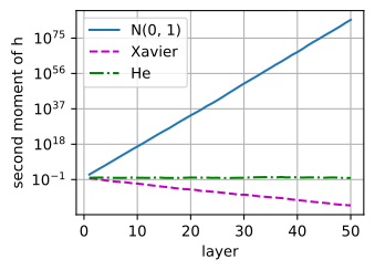
An unsuitable initialization can make gradients vanish or diverge before useful learning begins. In the examples below, ten sigmoid layers reduce the gradient to 10^{-6}; a hundred random matrices explode past 10^{24}; and one closing plot shows 10^{80} vs 10^{-15} vs flat (naive, Xavier, He).
The gradient is a product down the chain
Unstable Gradients
Backprop multiplies one Jacobian per layer. For a weight in layer \ell,
\partial_{\mathbf{W}^{(\ell)}} \mathbf{o} = \underbrace{\mathbf{M}^{(L)} \cdots \mathbf{M}^{(\ell+1)}}_{L-\ell \text{ Jacobians}}\, \mathbf{v}^{(\ell)}, \qquad \mathbf{M}^{(k)} = \partial_{\mathbf{h}^{(k-1)}} \mathbf{h}^{(k)}.
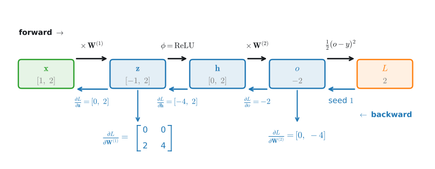
Forward pass builds z, h, o, L; the backward sweep multiplies a gradient back through every node.
Vanishing: the sigmoid saturates
Unstable Gradients · vanishing
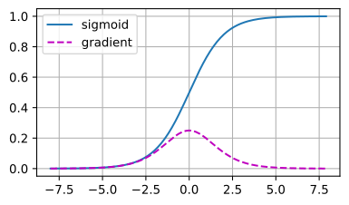
The sigmoid’s derivative peaks at 0.25 and is flat at zero in both tails.
Stack ten such layers and 0.25^{10} \approx 10^{-6}: the bottom layer sees a millionth of the gradient.
ReLU’s derivative is exactly 1 on active coordinates, so the activation does not attenuate gradients there. This property contributes to its use as a common default.
The demonstration: 10⁸⁰ vs 10⁻¹⁵ vs flat
Initialization · result
All three regimes in one plot: push a unit-scale signal through 50 ReLU layers and track E[(h^{(l)})^2] under three weight scales:
- \mathcal{N}(0,1): each layer gains \approx n_\textrm{in}/2 = 50\times; explodes to \sim\!10^{80}.
- Xavier: off by the rectifier’s \tfrac12 per layer; vanishes like 2^{-l} to \sim\!10^{-15}.
- He: essentially flat across all fifty layers.