Parameters from scratch

Implementation of Multilayer Perceptrons

Implementing an MLP two ways

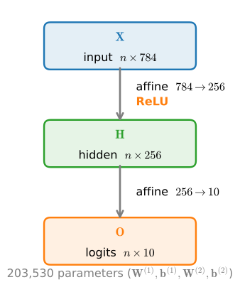
The simplest multilayer perceptron — two affine layers with a ReLU between them — trained end-to-end on Fashion-MNIST (28×28 grayscale, 10 classes).

  X (batch, 784)
       │ Linear  784 → 256
       │ ReLU
       │ Linear  256 → 10
       ▼
  logits (batch, 10)

We’ll build it twice — from scratch (manage the weights by hand) and concise (nn.Sequential) — to make concrete what the framework’s abstraction buys you.

Why one hidden layer of 256 is reasonable

For Fashion-MNIST (784 inputs → 10 outputs):

  • 256 hidden units = roughly 200k parameters. Big enough to memorize the training set in principle, small enough to actually train fast.
  • Powers of 2 for layer widths are a habit, not magic — matmul kernels are tuned for them; nothing breaks if you use 250 instead.
  • Single hidden layer because Fashion-MNIST is easy. A proper deep net wouldn’t help much without convolutions (next chapter).

These are hyperparameters — not learned. We set them by hand, train, and see what works.

Setup

from d2l import torch as d2l
import torch
from torch import nn

Two weight matrices, two bias vectors. Init: small Gaussian \mathcal{N}(0, \sigma^2) for weights, zero for biases.

\mathbf{W}^{(1)} \in \mathbb{R}^{784 \times 256},\quad \mathbf{b}^{(1)} \in \mathbb{R}^{256}, \mathbf{W}^{(2)} \in \mathbb{R}^{256 \times 10},\quad \mathbf{b}^{(2)} \in \mathbb{R}^{10}.

Total: 784 \cdot 256 + 256 + 256 \cdot 10 + 10 = 203\,530 parameters.

class MLPScratch(d2l.Classifier):
    def __init__(self, num_inputs, num_outputs, num_hiddens, lr, sigma=0.01):
        super().__init__()
        self.save_hyperparameters()
        self.W1 = nn.Parameter(torch.randn(num_inputs, num_hiddens) * sigma)
        self.b1 = nn.Parameter(torch.zeros(num_hiddens))
        self.W2 = nn.Parameter(torch.randn(num_hiddens, num_outputs) * sigma)
        self.b2 = nn.Parameter(torch.zeros(num_outputs))

ReLU and forward pass

First, our own ReLU — just max(X, 0) elementwise:

def relu(X):
    return torch.clamp(X, min=0)

Then the forward pass:

\mathbf{H} = \mathrm{ReLU}(\mathbf{X}\mathbf{W}^{(1)} + \mathbf{b}^{(1)}),\quad \mathbf{O} = \mathbf{H}\mathbf{W}^{(2)} + \mathbf{b}^{(2)}.

Image pixels are flattened to a 784-vector first — we’re ignoring spatial structure. (CNNs in the next chapter fix this.)

def forward(self, X):
    X = d2l.reshape(X, (-1, self.num_inputs))
    H = relu(d2l.matmul(X, self.W1) + self.b1)
    return d2l.matmul(H, self.W2) + self.b2

Training

Same Trainer, same Fashion-MNIST loaders, same cross-entropy loss as softmax regression. Only the model class changed:

model = MLPScratch(num_inputs=784, num_outputs=10, num_hiddens=256, lr=0.1)
data = d2l.FashionMNIST(batch_size=256)
trainer = d2l.Trainer(max_epochs=10)
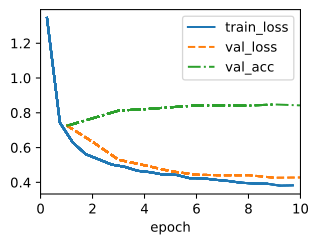
trainer.fit(model, data)

About 1–2 percentage points better than plain softmax regression on the same data. A nonlinearity earns its keep.

The concise version

Stack the same architecture using the framework’s container. Lazy linear layers infer input shapes; ReLU is built in:

class MLP(d2l.Classifier):
    def __init__(self, num_outputs, num_hiddens, lr):
        super().__init__()
        self.save_hyperparameters()
        self.net = nn.Sequential(nn.Flatten(), nn.LazyLinear(num_hiddens),
                                 nn.ReLU(), nn.LazyLinear(num_outputs))

That’s the whole architecture: 6 layers in a Sequential (Flatten + 2 Linear + 1 ReLU + glue), zero hand-rolled parameter management.

Both versions produce the same model. The framework just removes the bookkeeping.

Same training, same accuracy

model = MLP(num_outputs=10, num_hiddens=256, lr=0.1)
trainer.fit(model, data)
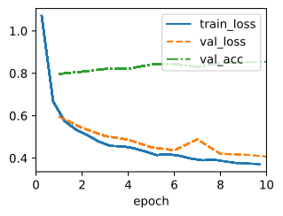
Identical convergence behavior. Built-in Linear and ReLU give you exactly what the from-scratch version computes — one of them is just easier to read and harder to bug.

What’s left to learn

We have a working MLP — but the real questions are open:

  • Initialization — pick \sigma so activations don’t explode or vanish through depth.
  • Generalization — why does it do well on unseen data?
  • Regularization — dropout, weight decay, etc.
  • Backprop — how gradients flow through arbitrary stacks.

Each is the topic of one of the next decks.

Recap

  • An MLP is a softmax classifier with one or more hidden layers + nonlinearity between affine transforms.
  • From scratch: 4 parameter tensors, hand-rolled ReLU, explicit matmuls. Useful to understand; tedious to ship.
  • Concise: Sequential(Flatten, Linear, ReLU, Linear) — same model, less bookkeeping.
  • Hyperparameters (depth, width, learning rate) live outside the model class; the same training loop works for any of them.
  • Beats softmax regression on Fashion-MNIST by a small but real margin — first taste of “depth helps”.