%matplotlib inline
from d2l import torch as d2l
import torch
from torch import nn
import pandas as pdKaggle in 30 seconds
The competition
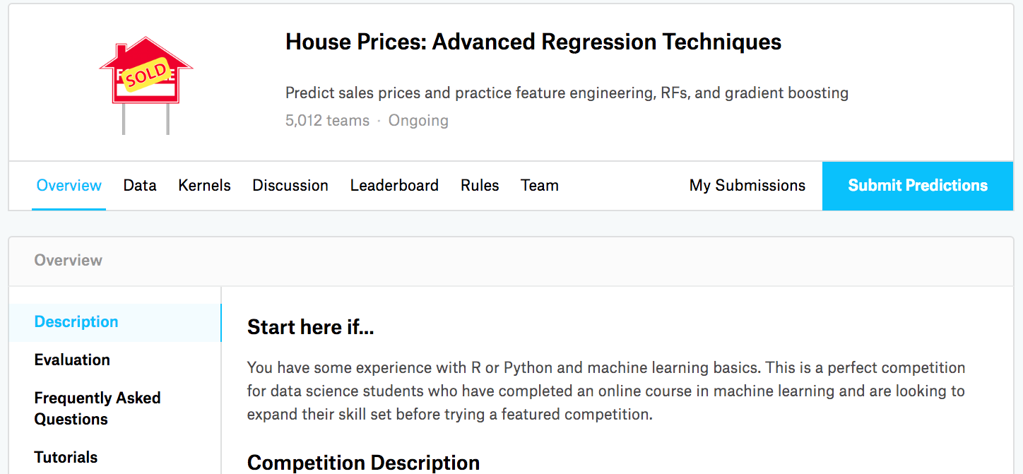
Kaggle hosts open ML competitions. Download the train and test CSVs, train locally, upload predictions, get scored on a held-out slice of the test set.
A public/private split on the test labels stops competitors from overfitting the leaderboard.

The House Prices competition page
The competition
The data contains no images, audio, or sequences, only a spreadsheet of house attributes and one price column.
This makes it a suitable first case study: the main work is the pipeline around the model.
K-fold cross-validation
Model selection
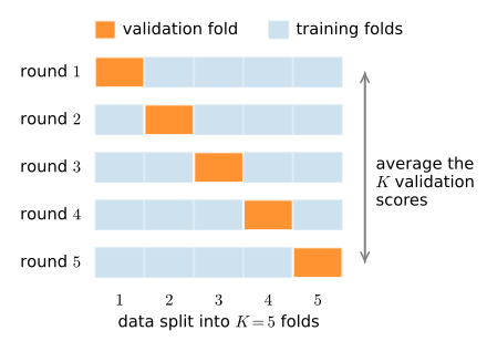
With ~1500 rows, one 80/20 split is noisy. Split the data into K folds; train K times, each time holding out a different fold; average the K validation scores.
This costs K\times the compute but provides a more stable estimate, and the same loop supports hyperparameter search. Fit preprocessing anew inside each training fold; otherwise the held-out fold leaks into the model pipeline.
An underfit baseline gives a misleading comparison
Model selection
Start with a linear model, a fast baseline, but train it competently: 100 epochs at lr 0.03, not the customary ten. Ten epochs of SGD on these features leaves it badly underfit.
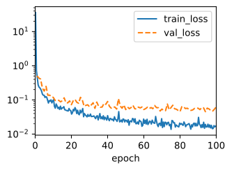
fold validation log mse = [0.0457, 0.0303, 0.0480, 0.0331, 0.0178]
mean = 0.0350; sd = 0.0123
In these runs, ten epochs leave the linear model underfit whereas the longer run reaches about 0.036. Comparisons should use a baseline with a validated training budget.
Cross-validation comparison
Model selection
Same K-fold loop, learning rate, and epoch budget, only the model changes:
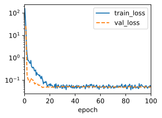
fold validation log mse = [0.0506, 0.0276, 0.0538, 0.0188, 0.0289]
mean = 0.0359; sd = 0.0154
For these configurations, the fold means are about 0.036 linear vs 0.027 MLP. Fold dispersion and model-specific tuning are needed to assess the difference; a tree model remains an untested baseline.
Submit: ensemble the folds, write the CSV
Submitting
Average the K log-price predictions, exponentiate, submit:
for model, _ in models:
    model.eval()  # already the case after Trainer.fit; explicit is safer
preds = [model(d2l.tensor(test.values.astype(float), dtype=d2l.float32))
         for model, test in models]
# Each model predicts a log-price; average across the K folds in log space,
# then exponentiate back to a price.
ensemble_preds = d2l.exp(d2l.reduce_mean(d2l.concat(preds, 1), 1))
submission = pd.DataFrame({'Id':data.raw_val.Id,
                           'SalePrice':d2l.numpy(ensemble_preds)})
submission.to_csv('submission.csv', index=False)
The log-space mean averages predictions in the space where RMSLE measures error; exponentiating makes it a geometric mean in price space. This does not guarantee an improvement. The CV score measured a single fold model; refitting on all data is the more direct alternative to this fold ensembling.