Implementing it

Dropout

Dropout regularizes by thinning

Dropout (Srivastava, Hinton et al., 2014) is the simplest and most widely used regularizer for neural networks:

During training, set each hidden unit to zero independently with probability p. Rescale the survivors by 1/(1-p). Turn it off at test time.

Counterintuitive — we actively damage the network mid-training — but the trick is rock-solid. It still ships in modern Transformers (~10% rate standard).

Why we need it

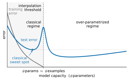
Modern networks are overparameterized — more weights than training examples. Without a regularizer, gradient descent happily memorizes the training set.

Two complementary reasons dropout helps:

• Noise injection = smoothness regularization (Bishop 1995). Robustness to hidden-unit dropout forces the network to be a smoother function of its inputs.
• Anti-co-adaptation: a unit can’t rely on any specific upstream unit being present, so it picks up signal from a broader, redundant set of features.

What dropout looks like

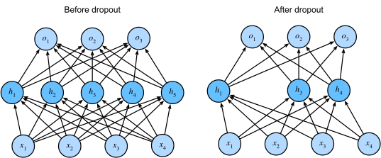
On every minibatch we randomly zero a fraction of hidden units; the network on this iteration is a thinned subnetwork. Across iterations we sample many subnetworks:

Two of the five hidden units zeroed by a single dropout draw. Each iteration samples a different subset.

At test time dropout is off — we use the full network. Effectively we average exponentially many thinned subnetworks (a kind of cheap ensemble).

The arithmetic: keep the expectation

Per hidden unit h, replace with

h' = \begin{cases} 0 & \text{with probability } p, \\ \dfrac{h}{1 - p} & \text{otherwise.} \end{cases}

The rescaling 1/(1-p) is what makes \mathbb{E}[h'] = h. Without it, expected activations shrink by (1-p) during training but recover their full scale at test time → train/test mismatch.

This is “inverted dropout”; the version every modern framework uses.

Setup

from d2l import torch as d2l
import torch
from torch import nn

Sample a Bernoulli mask, multiply, rescale:

def dropout_layer(X, dropout):
    assert 0 <= dropout <= 1
    if dropout == 1: return torch.zeros_like(X)
    mask = (torch.rand(X.shape) > dropout).float()
    return mask * X / (1.0 - dropout)

Quick check on a 2×8 input:

X = torch.arange(16, dtype = torch.float32).reshape((2, 8))
print('dropout_p = 0:', dropout_layer(X, 0))
print('dropout_p = 0.5:', dropout_layer(X, 0.5))
print('dropout_p = 1:', dropout_layer(X, 1))

dropout_p = 0: tensor([[ 0.,  1.,  2.,  3.,  4.,  5.,  6.,  7.],
        [ 8.,  9., 10., 11., 12., 13., 14., 15.]])
dropout_p = 0.5: tensor([[ 0.,  2.,  4.,  0.,  0., 10., 12., 14.],
        [ 0., 18., 20., 22.,  0.,  0., 28.,  0.]])
dropout_p = 1: tensor([[0., 0., 0., 0., 0., 0., 0., 0.],
        [0., 0., 0., 0., 0., 0., 0., 0.]])

• p = 0 → identity (no dropout).
• p = 0.5 → about half the entries zero, the rest doubled.
• p = 1.0 → all zeros (degenerate).

Where to put dropout

After the activation, before the next linear layer:

Linear → ReLU → Dropout(p₁) → Linear → ReLU → Dropout(p₂) → Linear

Convention: less on early layers (low-level features need to be reliable), more later (high-level features overfit).

Typical values:

• MLPs / Transformers: 0.1–0.5.
• CNNs: 0–0.2 (BatchNorm largely supplants dropout).
• Just before the classifier head: 0.5 is standard.

MLP with dropout

class DropoutMLPScratch(d2l.Classifier):
    def __init__(self, num_outputs, num_hiddens_1, num_hiddens_2,
                 dropout_1, dropout_2, lr):
        super().__init__()
        self.save_hyperparameters()
        self.lin1 = nn.LazyLinear(num_hiddens_1)
        self.lin2 = nn.LazyLinear(num_hiddens_2)
        self.lin3 = nn.LazyLinear(num_outputs)
        self.relu = nn.ReLU()

    def forward(self, X):
        H1 = self.relu(self.lin1(X.reshape((X.shape[0], -1))))
        if self.training:  
            H1 = dropout_layer(H1, self.dropout_1)
        H2 = self.relu(self.lin2(H1))
        if self.training:
            H2 = dropout_layer(H2, self.dropout_2)
        return self.lin3(H2)

Training

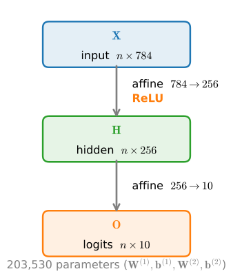
Two hidden layers (256 each), dropout 0.5 between them:

hparams = {'num_outputs':10, 'num_hiddens_1':256, 'num_hiddens_2':256,
           'dropout_1':0.5, 'dropout_2':0.5, 'lr':0.1}
model = DropoutMLPScratch(**hparams)
data = d2l.FashionMNIST(batch_size=256)
trainer = d2l.Trainer(max_epochs=10)
trainer.fit(model, data)

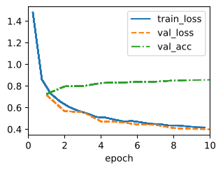
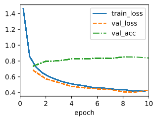
Validation accuracy is better than the plain MLP from the previous deck — the gap between train and test loss shrinks visibly. Dropout shines when capacity exceeds the data.

Framework version

nn.Dropout(p) is a stock layer. It also handles the train vs. eval mode switch — call model.eval() and dropout becomes a no-op:

class DropoutMLP(d2l.Classifier):
    def __init__(self, num_outputs, num_hiddens_1, num_hiddens_2,
                 dropout_1, dropout_2, lr):
        super().__init__()
        self.save_hyperparameters()
        self.net = nn.Sequential(
            nn.Flatten(), nn.LazyLinear(num_hiddens_1), nn.ReLU(), 
            nn.Dropout(dropout_1), nn.LazyLinear(num_hiddens_2), nn.ReLU(), 
            nn.Dropout(dropout_2), nn.LazyLinear(num_outputs))

model = DropoutMLP(**hparams)
trainer.fit(model, data)

Why dropout works (the modern view)

Several complementary explanations, none complete on its own:

• Bayesian model averaging — training samples a different thinned network each step; testing averages \sim 2^n subnetworks → cheap ensemble.
• Stochastic regularization — equivalent to adding Gaussian noise; Bishop showed this is Tikhonov (\ell_2) regularization on the function.
• Anti-co-adaptation — forces redundant features.
• Variance bound — caps the variance the network puts into any one direction in feature space.

Dropout in 2026

Modern deep nets often replace dropout with BatchNorm / LayerNorm, which provides similar regularization “for free”.

But dropout remains alive and well:

• Transformers — rate 0.1 by default in attention and FFN sublayers.
• Final classifier heads — 0.5 right before the output projection is still a standard recipe.

Recap

• Dropout: zero each hidden unit with prob p during training; rescale survivors by 1/(1-p) to preserve expectations.
• Off at test time — full network in use.
• Place after activation, before next linear layer; rates 0.1–0.5 typical.
• Equivalent to (a) injecting noise = smoothness regularization, and (b) ensembling exponentially many thinned subnetworks.
• One of the cheapest, most reliable regularizers — combines well with weight decay, layer norm, and data augmentation.