Random Variables

Dive into Deep Learning · §26.1

Densities, moments, and joint distributions
the continuous language of deep learning.

Why continuous probability?

Motivation

Pixels, weights, activations, and noise are all continuous. A single exact outcome now has probability zero: probability lives in areas, not points.

Density p, mean, variance, covariance, the matrix \boldsymbol\Sigma.
The toolkit behind SGD, normalizing flows, and Bayesian inference.

The continuous analogue of discrete probability: same ideas, integration in place of summation.

Densities and the c.d.f.

the dartboard argument, p\ge 0, \int p = 1, and F' = p

The density appears

The dartboard

Shrink the bin around x by 10\times and the probability it catches shrinks by 10\times. The surviving constant of proportionality is the density:

P\bigl(X \in [x, x+\epsilon]\bigr) \approx \epsilon\, p(x).

So P(X = x) = 0 for every fixed point, and p(x) may exceed 1: a density is a rate, not a probability.

Probability is area

Two defining properties

A density is non-negative and integrates to one; probability of an interval is the area beneath it:

p(x)\ge 0, \qquad \int_{-\infty}^{\infty} p(x)\,dx = 1, \qquad P\bigl(X\in(a,b]\bigr) = \int_a^b p(x)\,dx.

A Riemann sum over a two-bump mixture confirms the total mass is 1 and recovers P(-2 < X \le 3) from the density alone:

total mass     : 1.0000
P(-2 < X <= 3) : 0.7725

The c.d.f. and the FTC

The c.d.f.

The cumulative distribution accumulates the density, F(x) = \int_{-\infty}^x p = P(X \le x), rising monotonically from 0 to 1. The same number two ways: the area under p over (a,b] equals the rise F(b)-F(a).

Proposition. If p is continuous, F'(x) = p(x): the density is the slope of the c.d.f. (fundamental theorem of calculus).

The quantile function is a sampler

The c.d.f.

The c.d.f. covers every kind of variable (staircase, smooth curve, mixture), and its inverse F^{-1}(q), the quantile function, turns uniform noise into samples from any distribution:

Proposition (inverse transform). If U\sim\mathrm{Uniform}[0,1], then X = F^{-1}(U) has c.d.f. F. Proof. \{F^{-1}(U)\le x\} = \{U \le F(x)\}, and the uniform gives that event probability F(x). \blacksquare

Where F is steep (where the density is large), uniform levels land densely: the slope does the shaping.

Mean, variance, and tail bounds

linearity, the computational form, Markov, Chebyshev

The mean is linear

Moments

The mean is the density-weighted center, \mu_X = \mathbb E[X] = \int x\,p(x)\,dx.

Proposition. \mathbb E[aX+b] = a\,\mathbb E[X] + b and \mathbb E[X+Y] = \mathbb E[X] + \mathbb E[Y] (no independence needed).

The sum rule follows by splitting the joint expectation through the marginals; it is why we can move \mathbb E freely through a network’s losses.

Variance and its computational form

Moments

Variance is the mean squared deviation, \sigma_X^2 = \mathbb E[(X-\mu_X)^2].

Proposition. \operatorname{Var}(X) = \mathbb E[X^2] - \mu_X^2 and \operatorname{Var}(aX+b) = a^2\operatorname{Var}(X).

Proof. Expand (X-\mu_X)^2 = X^2 - 2\mu_X X + \mu_X^2 and take expectations. A shift b cancels inside the deviation a(X-\mu_X), so only a^2 survives the square. \blacksquare

Markov’s inequality

Tail bounds

For a non-negative X and any a>0,

P(X \ge a) \le \frac{\mathbb E[X]}{a}.

Proof. Pointwise X \ge a\,\mathbf 1_{\{X\ge a\}}; take expectations and use \mathbb E[\mathbf 1_{\{X\ge a\}}] = P(X\ge a). \blacksquare

No distributional assumption at all: it bounds gradient norms, incomes, and file sizes alike.

Chebyshev: σ sets the scale

Tail bounds

Standard deviation measures distance in universal units:

P\bigl(|X-\mu_X| \ge \alpha\,\sigma_X\bigr) \le \frac{1}{\alpha^2}.

Proof. Apply Markov to Z = (X-\mu_X)^2 with a = \alpha^2\sigma_X^2. \blacksquare

The bound is sharp: the three-atom example attains equality at p=\tfrac18.

When moments fail: Cauchy

Counterexample

For p(x) = \dfrac{1}{\pi(1+x^2)} both summaries fail, at two speeds. The variance integrand tends to \tfrac1\pi, so \int_{-R}^{R} x^2 p\,dx = \tfrac{2}{\pi}(R - \arctan R) grows linearly, multiplying by ten per decade:

integral_-10^10 x^2 p(x) dx = 5.430
integral_-100^100 x^2 p(x) dx = 62.668
integral_-1000^1000 x^2 p(x) dx = 635.620

The mean fails more subtly: the odd integrand tempts “0 by symmetry,” but a mean needs \int |x|\,p\,dx < \infty, and that integral diverges like \tfrac{1}{\pi}\log(1+R^2). The mean is a meaningless \infty - \infty whose value depends on how the limits are taken. Absolute integrability is what a finite mean requires; symmetry alone proves nothing.

Several variables

marginals, conditioning, covariance, change of variables

Joint and marginal densities

Several variables

A joint density p(x,y)\ge 0 integrates to 1 over the plane. Marginalize by integrating out the variable you do not care about:

p_X(x) = \int_{-\infty}^{\infty} p_{X,Y}(x,y)\,dy.

Integrate the joint up a vertical strip at x to get the marginal height there.

Conditioning and independence

Conditioning

Slice the joint at Y=y and renormalize:

p_{X\mid Y}(x\mid y) = \frac{p_{X,Y}(x,y)}{p_Y(y)}.

Chain rule p_{X,Y} = p_{X\mid Y}\,p_Y gives Bayes’ rule for densities. X \perp Y exactly when the joint factorizes: the slice shape stops depending on y.

Conditional expectation & the tower

Conditioning

\mathbb E[X\mid Y=y] = \int x\,p_{X\mid Y}(x\mid y)\,dx averages within a slice.

Tower / Eve’s law. \mathbb E[X] = \mathbb E\bigl[\mathbb E[X\mid Y]\bigr] and \operatorname{Var}(X) = \mathbb E[\operatorname{Var}(X\mid Y)] + \operatorname{Var}(\mathbb E[X\mid Y]).

Total variance = unexplained (within-slice spread) + explained (spread of slice means): the decomposition behind ANOVA and latent-variable models.

Covariance

Co-variation

\operatorname{Cov}(X,Y) = \mathbb E[XY] - \mathbb E[X]\,\mathbb E[Y] measures linear co-variation, in mixed units:

\operatorname{Var}(X+Y) = \operatorname{Var}(X) + \operatorname{Var}(Y) + 2\operatorname{Cov}(X,Y).

Zero covariance is weaker than independence: with Y uniform on \{-2,\dots,2\} and X=Y^2, covariance is 0 yet X is a function of Y.

Correlation is a cosine

Co-variation

Normalize covariance to kill the units: \rho = \operatorname{Cov}(X,Y)/(\sigma_X\sigma_Y) \in [-1,1].

Proof of the bound. \operatorname{Var}(tX+Y)\ge 0 is a non-negative quadratic in t; its discriminant gives \operatorname{Cov}^2 \le \operatorname{Var}(X)\operatorname{Var}(Y), with equality iff Y = aX+b. \blacksquare

So \rho = \cos\theta between centered variables, by the same Cauchy–Schwarz argument.

The covariance matrix → PCA

Co-variation

Stack pairwise covariances into \Sigma_{ij} = \operatorname{Cov}(X_i,X_j). It is symmetric and positive semidefinite, since \mathbf a^\top\Sigma\,\mathbf a = \operatorname{Var}\bigl(\textstyle\sum_i a_i X_i\bigr) \ge 0.

Gaussian contours are ellipses whose axes are the eigenvectors of \Sigma with half-lengths \propto\sqrt{\lambda_i}: finding them is PCA (the spectral theorem in action).

Change of variables for densities

Pushforward

Map Y=g(X). To conserve probability, density thins by the local stretch:

p_Y(y) = p_X\bigl(g^{-1}(y)\bigr)\,\left|\frac{dg^{-1}}{dy}(y)\right|.

In many dimensions this becomes a log-determinant of the Jacobian:

\log p_Y(\mathbf y) = \log p_X(\mathbf x) - \log\bigl|\det J_g(\mathbf x)\bigr|.

Log-dets add under composition → a normalizing flow stacks layers and just sums one -\log|\det J_g| per layer.

Change of variables, verified

Pushforward

For X\sim\mathcal N(0,1) and Y = e^X, the formula gives the log-normal p_Y(y) = \tfrac{1}{y\sqrt{2\pi}}\exp\!\bigl(-\tfrac12(\log y)^2\bigr), and a histogram of e^X matches it exactly:

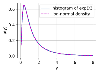
The naive guess p_X(\log y) peaks at y=1; the Jacobian correction moves the true peak to y=e^{-1}.

Recap

Wrap-up

Density p\ge 0, \int p = 1; probability is area; F'=p (FTC).
\mathbb E is linear (no independence); \operatorname{Var}=\mathbb E[X^2]-\mu^2.
Chebyshev: P(|X-\mu|\ge\alpha\sigma)\le1/\alpha^2 for any distribution, and it is sharp.
Cauchy: a finite mean needs \int|x|\,p\,dx<\infty; symmetry alone proves nothing.

Marginalize by integrating out; condition by slicing + renormalizing; Bayes for densities.
Tower / Eve: total = explained + unexplained variance.
Covariance is linear co-variation; correlation is its cosine in [-1,1]; \Sigma\succeq 0 → ellipse axes = PCA.
Change of variables: the Jacobian keeps mass; log-dets sum → normalizing flows.

Next: the named distributions, the specific shapes this machinery describes.