Distributions

Dive into Deep Learning · §26.2

The distributions a practitioner needs
from Bernoulli to the Gaussian, and the family they belong to.

A family, not a list

Motivation

Fourteen distributions cover almost everything in practice, and they connect: Bernoulli is the seed; construction and limit arrows grow the rest; conjugate priors close the tree, all inside one envelope.

Learn the map, not a flat list of formulas.

01

Discrete distributions

Bernoulli · Categorical · Uniform · Binomial · Poisson

Bernoulli: the seed

Discrete

One coin flip: P(X=1)=p, P(X=0)=1-p. Because X^2 = X, both moments collapse instantly: \mathbb E[X]=p, \operatorname{Var}(X)=p(1-p).

import numpy as onp
rng = onp.random.default_rng(0)
p = 0.3
sample = 1 * (rng.random((3, 3)) < p)          # 1 with prob p, else 0
big = 1 * (rng.random(10000) < p)              # large sample for the mean
print('pmf  P(0), P(1) =', (1 - p, p))
print('mean of 10,000 draws =', float(big.mean()), ' (≈ p)')
sample

pmf  P(0), P(1) = (0.7, 0.3)
mean of 10,000 draws = 0.3006  (≈ p)
array([[0, 1, 1],
       [1, 0, 0],
       [0, 0, 0]])

Every binary classifier outputs a Bernoulli; its negative log-likelihood is binary cross-entropy.

Categorical: softmax in disguise

Discrete

K outcomes with P(X=k)=p_k. A network produces the p_k from logits through the softmax p_k = e^{z_k}/\sum_j e^{z_j}, and the NLL is exactly cross-entropy.

import numpy as onp
rng = onp.random.default_rng(0)
z = onp.array([2.0, 1.0, 0.1, -1.0])            # logits over K = 4 classes
p_cat = onp.exp(z) / onp.exp(z).sum()            # softmax -> categorical
draw = int(rng.choice(len(p_cat), p=p_cat))
print('categorical p =', p_cat.round(3), ' sum =', float(p_cat.sum()))
print('one sample -> class', draw)

categorical p = [0.638 0.235 0.095 0.032]  sum = 1.0
one sample -> class 0

The Gumbel-max trick samples a categorical exactly; its soft version makes discrete choices differentiable.

The discrete gallery

Discrete

Four laws in one picture, mass on the integers:

Uniform spreads mass evenly (\mu=\tfrac{n+1}{2}); the others concentrate it where events are likely.

Binomial: moments for free

Discrete

A Binomial is a sum of n Bernoullis, X=\sum_i X_i, so linearity and independence hand us the moments with no algebra:

\mu = \sum_i \mathbb E[X_i] = np, \qquad \sigma^2 = \sum_i \operatorname{Var}(X_i) = np(1-p).

mean onp = 4.0   var onp(1-p) = 2.4
P(X=k): [0.006 0.04  0.121 0.215 0.251 0.201 0.111 0.042 0.011 0.002 0.   ]
array([[5, 3, 1],
       [1, 5, 6],
       [4, 5, 4]])

Poisson: the many-rare limit

Discrete

Take \text{Binomial}(n,\lambda/n) and send n\to\infty:

\binom{n}{k}\Bigl(\tfrac{\lambda}{n}\Bigr)^k\Bigl(1-\tfrac{\lambda}{n}\Bigr)^{n-k} \longrightarrow \frac{\lambda^k e^{-\lambda}}{k!}.

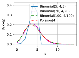
Mean = variance =\lambda is the Poisson fingerprint: over-dispersion (variance > mean) signals a too-simple model.

02

Continuous distributions

Uniform · Exponential · Gaussian · Laplace · Multivariate Gaussian

Uniform: raw randomness

Continuous

Density \tfrac{1}{b-a} on [a,b]; mean \tfrac{a+b}{2}, variance \tfrac{(b-a)^2}{12}.

The unit uniform powers inverse-transform sampling, Monte Carlo, dropout masks, and initialization.

rng = np.random.default_rng(0)
a, b = 1.0, 3.0
sample = (b - a) * rng.random(10000) + a         # shift-and-scale U(0,1)
print('mean (a+b)/2   =', (a + b) / 2, '  sample mean:',
      float(sample.mean().round(3)))
print('var (b-a)^2/12 =', round((b - a)**2 / 12, 3), ' sample var :',
      float(sample.var().round(3)))

mean (a+b)/2   = 2.0   sample mean: 1.999
var (b-a)^2/12 = 0.333  sample var : 0.334

Exponential: memorylessness

Continuous

Waiting times: p(x)=\lambda e^{-\lambda x}, F(x)=1-e^{-\lambda x}, mean 1/\lambda, variance 1/\lambda^2.

P(X > s+t \mid X > s) = e^{-\lambda t} = P(X > t).

import numpy as onp
rng = onp.random.default_rng(0)
lam = 0.5
U = rng.random(100000)
sample = -onp.log(U) / lam                        # inverse-transform sampler
print('mean 1/lambda =', 1 / lam, '  sample mean =', float(sample.mean().round(3)))
print('var 1/lambda^2 =', 1 / lam**2, ' sample var =', float(sample.var().round(3)))

mean 1/lambda = 2.0   sample mean = 2.001
var 1/lambda^2 = 4.0  sample var = 3.984

The only memoryless continuous law (converse: Exercise 4); the continuous partner of the Poisson, and the source of X=-\log U/\lambda sampling.

Gaussian: the CLT limit

Continuous

Standardized sums of any iid finite-variance terms converge to the Gaussian. Watch universality happen, starting from the least Gaussian summand available, the flat, hard-edged uniform:

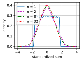
n=1 is a plateau, n=2 a triangle; by n=32 the sum is indistinguishable from \mathcal N(0,1) at this resolution. Nothing in the code knows about the Gaussian: summation manufactures it. (It is also the maximum-entropy law for fixed mean and variance.)

The normalizer: a polar trick

Continuous

Why \sqrt{2\pi}? Recall from the integral-calculus chapter: square the integral and switch to polar coordinates,

I^2 = \!\int\!\!\int e^{-(x^2+y^2)/2}\,dx\,dy = \!\int_0^{2\pi}\!\!\int_0^{\infty} e^{-r^2/2}\,r\,dr\,d\theta = 2\pi.

The Jacobian factor r makes the radial integral elementary, so I=\sqrt{2\pi}; the full derivation lives in the integral-calculus chapter.

Laplace: the L1 sibling

Continuous

p(x)=\tfrac{1}{2b}e^{-|x-\mu|/b}: a sharp peak and heavier (exponential) tails than the Gaussian; variance 2b^2.

import numpy as onp
rng = onp.random.default_rng(0)
mu, b = 0.0, 1.0
sigma = onp.sqrt(2) * b                            # matched-variance Gaussian sd
U = (rng.random(200000) - 0.5) * (1 - 1e-7)       # open interval avoids log(0)
lap = mu - b * onp.sign(U) * onp.log(1 - 2 * onp.abs(U))  # inverse transform
gau = rng.normal(mu, sigma, 200000)
print('Laplace var (2b^2):', float(lap.var().round(3)), ' Gaussian var:', float(gau.var().round(3)))
print('P(|x| > 3sd): Laplace', float((onp.abs(lap) > 3 * sigma).mean()),
      ' Gaussian', float((onp.abs(gau) > 3 * sigma).mean()))

Laplace var (2b^2): 1.998  Gaussian var: 2.005
P(|x| > 3sd): Laplace 0.014575  Gaussian 0.00272

Its NLL is |y-\hat y| (MAE); as a prior it gives the \ell_1 / LASSO penalty; its ML location estimator is the median, not the mean.

Multivariate Gaussian: covariance geometry

Continuous

p(\mathbf x)\propto \exp\!\Bigl(-\tfrac12(\mathbf x-\boldsymbol\mu)^\top \boldsymbol\Sigma^{-1}(\mathbf x-\boldsymbol\mu)\Bigr).

Contours are ellipsoids: axes along the eigenvectors of \boldsymbol\Sigma, half-lengths \propto\sqrt{\lambda_i}. Isotropy = spheres = independent coordinates. Sampling is the Cholesky recipe: \boldsymbol\Sigma=\mathbf L\mathbf L^\top, \mathbf x=\boldsymbol\mu+\mathbf L\mathbf z.

empirical covariance:
 [[1.96 1.03]
 [1.03 2.06]]
eigenvalues (≈ 1, 3): [0.98 3.04]
Cholesky-recipe covariance:
 [[1.93 0.97]
 [0.97 2.  ]]

Closed under conditioning

Continuous

Partition \mathbf x=(\mathbf x_1,\mathbf x_2). Then \mathbf x_1\mid\mathbf x_2 is Gaussian with

\boldsymbol\mu_{1\mid 2} = \boldsymbol\mu_1 + \boldsymbol\Sigma_{12}\boldsymbol\Sigma_{22}^{-1}(\mathbf x_2-\boldsymbol\mu_2), \quad \boldsymbol\Sigma_{1\mid 2} = \boldsymbol\Sigma_{11} - \boldsymbol\Sigma_{12}\boldsymbol\Sigma_{22}^{-1}\boldsymbol\Sigma_{21}.

Conditional mean is linear in \mathbf x_2; the Schur-complement covariance is the entire engine of Gaussian-process regression.

In high dimension, the Gaussian is a thin shell

Continuous

\|\mathbf x\|^2 sums d independent mean-1 terms, so it concentrates near d: the mass lives in a shell of radius \approx\sqrt d, far from the origin where the density is pointwise largest; and two independent draws are nearly orthogonal, cosine \sim 1/\sqrt d:

d =   3:  ||x||/sqrt(d) = 0.920 ± 0.378,   mean |cos(x,y)| = 0.497
d =  30:  ||x||/sqrt(d) = 0.992 ± 0.127,   mean |cos(x,y)| = 0.145
d = 300:  ||x||/sqrt(d) = 1.000 ± 0.039,   mean |cos(x,y)| = 0.046

Load-bearing facts: 1/\sqrt d initialization keeps \|\mathbf{Wx}\|\approx\|\mathbf x\|; cosine similarity is informative because unrelated vectors sit near 0; nearest-neighbor contrast fades. Exponential tail bounds arrive in the concentration-and-generalization section.

03

The exponential family

one form, maximum entropy, the moment property

One shared form

Unification

p(\mathbf x\mid\boldsymbol\eta) = h(\mathbf x)\, \exp\!\bigl(\boldsymbol\eta^\top T(\mathbf x) - A(\boldsymbol\eta)\bigr).

Base measure h, natural parameters \boldsymbol\eta, sufficient statistics T, log-partition A. Bernoulli (\eta=\operatorname{logit}p, A=\operatorname{softplus}), Poisson (\eta=\log\lambda), and Gaussian all fit.

Two exclusions, two reasons: the uniforms stay outside because their support moves with the parameters; Cauchy and Student-t do not admit a fixed finite-dimensional sufficient statistic for their usual unknown location-and-scale families. They therefore lack the standard finite-dimensional conjugate update, and their negative log-likelihoods are not generally convex.

Where the form comes from

Unification

Maximize entropy H_h[p] subject to fixed averages \mathbb E[T(\mathbf x)] = \boldsymbol\tau. The Lagrange multipliers are the natural parameters, and the maximizer is exactly p\propto h\,e^{\boldsymbol\eta^\top T}.

The exponential family is the least-committal family consistent with a chosen set of expected statistics.

The moment property

Unification

Differentiating the log-partition recovers the moments:

\nabla A(\boldsymbol\eta) = \mathbb E[T(\mathbf x)], \qquad \nabla^2 A(\boldsymbol\eta) = \operatorname{Cov}(T) \succeq 0.

So A is convex and the MLE equation is moment matching, \mathbb E[T] = \bar T. Autograd confirms dA/d\eta=\sigma(\eta) for the Bernoulli:

import numpy as onp
eta = 0.7                                        # natural parameter (logit)
A = lambda e: onp.log1p(onp.exp(e))                # Bernoulli log-partition (softplus)
eps = 1e-6
dA = (A(eta + eps) - A(eta - eps)) / (2 * eps)   # numerical dA/deta
print('dA/deta      =', round(float(dA), 6))
print('sigmoid(eta) = E[x] = p =', round(float(1 / (1 + onp.exp(-eta))), 6))

dA/deta      = 0.668188
sigmoid(eta) = E[x] = p = 0.668188

04

Conjugate priors

Beta · Gamma · Dirichlet: updating is counting

Beta–Bernoulli: pseudo-counts

Priors

A \text{Beta}(\alpha,\beta) prior times a Bernoulli likelihood with x heads in n flips gives a \text{Beta}(\alpha+x,\beta+n-x) posterior; \alpha,\beta act as phantom heads and tails:

\mathbb E[\theta\mid X] = \frac{\alpha+x}{\alpha+\beta+n}.

prior mean      = 0.5
MLE  x/n        = 0.7
posterior Beta  = (9.0, 5.0)
posterior mean  = 0.6429

\alpha=\beta=1 recovers Laplace’s rule of succession (x+1)/(n+2).

The rest of the tier

Priors

Gamma → Poisson. Pseudo-events over a pseudo-window; marginalizing the rate gives the over-dispersed negative binomial.

Dirichlet → Categorical. A multivariate Beta: one pseudo-count per class on the simplex.

General fact. Every exponential-family likelihood has a conjugate prior of the same form; its hyperparameters are pseudo-data (\boldsymbol\nu,\kappa).

Recap

Wrap-up

• Bernoulli → Binomial → Poisson / Gaussian by sums and limits; Categorical → Multinomial.
• Moments from linearity, limits, and a few integrals.
• Gaussian is central: CLT, max entropy, closed under linear maps and conditioning (Schur complement).

• The exponential family unifies them; \nabla A=\mathbb E[T], and its NLL is convex in natural parameters.
• The usual conjugate families (Beta / Gamma / Dirichlet) update by adding sufficient statistics.
• The named shapes are the vocabulary; maximum likelihood is the grammar (next).