def mutual_information(p_xy):
"""I(X;Y) of a discrete joint p.m.f., in nats."""
p_x = p_xy.sum(axis=1, keepdims=True) # marginals from the joint
p_y = p_xy.sum(axis=0, keepdims=True)
return float((p_xy * onp.log(p_xy / (p_x * p_y))).sum())
mi_kl = mutual_information(p_xy) # divergence form
mi_ent = H_x + H_y - H_xy # entropy identity
print(f'I(X;Y) = {mi_kl:.4f} nats (KL form) '
f'= {mi_ent:.4f} nats (entropy identity)')
print(f' = {mi_kl / onp.log(2):.4f} bits')Mutual Information and Representation Learning
Dive into Deep Learning · §28.3
How far is a pair from independent?
mutual information and the objectives of representation learning.
Mutual information: distance from independence
Motivation
I(X;Y) = D_{\mathrm{KL}}(P_{X,Y}\,\|\,P_X\otimes P_Y): how far the joint sits from the product of its marginals. Symmetric, \ge 0, zero iff independent, and
I = H(X) - H(X\mid Y) = H(X)+H(Y)-H(X,Y).
01
The calculus of dependence
entropy bookkeeping, invariance, and the data-processing inequality
Joint and conditional entropy
Bookkeeping
The chain rule H(X,Y) = H(X) + H(Y\mid X) is an accounting identity: the surprise of the pair is the surprise of X plus the residual in Y:
marginals: p_x = [0.5 0.5], p_y = [0.3 0.7]
H(X,Y) = 1.2799, H(X) = 0.6931, H(Y) = 0.6109 nats
H(Y|X) = 0.5867 = H(X,Y) - H(X) = 0.5867 nats
Every entropy quantity, one concrete number.
Equivalent definitions of mutual information
Definition
The shared area of the entropy diagram, computed two ways (the KL-from- independence form and the entropy identity), gives the same numerical value:
I(X;Y) = 0.0242 nats (KL form) = 0.0242 nats (entropy identity)
       = 0.0349 bits
Symmetry and I \ge 0 are immediate from Gibbs.
The Gaussian anchor
Ground truth
Ground truth is I = -\tfrac12\log(1-\rho^2), yet a histogram is already biased at \rho=0.99:
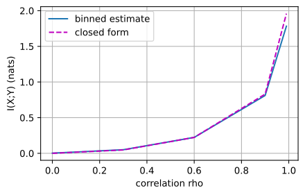
rho = 0.00: binned = 0.0027, closed form = -0.0000 nats
rho = 0.30: binned = 0.0504, closed form = 0.0472 nats
rho = 0.60: binned = 0.2235, closed form = 0.2231 nats
rho = 0.90: binned = 0.8111, closed form = 0.8304 nats
rho = 0.99: binned = 1.7829, closed form = 1.9585 nats
MI sees what correlation cannot
Nonlinear dependence
Correlation measures only linear association. With Y = X^2 + \text{noise}, \rho \approx 0 yet I \approx 1 nat, and MI is invariant to any invertible reparameterization:
rng = onp.random.default_rng(0)
n = 200_000
x = rng.standard_normal(n)
y = x**2 + 0.3 * rng.standard_normal(n)    # zero correlation by symmetry

print(f'sample correlation rho = {onp.corrcoef(x, y)[0, 1]:+.4f}')
print(f'binned MI estimate     = {binned_mi(x, y):.4f} nats')
print(f'after x -> 2x + 3      = {binned_mi(2 * x + 3, y):.4f} nats')
sample correlation rho = -0.0028
binned MI estimate = 0.9814 nats
after x -> 2x + 3 = 0.9814 natsPointwise MI ranks co-occurrences
PMI
\mathrm{pmi}(x,y) = \log\frac{p(x,y)}{p(x)\,p(y)} scores a single pair, and I = \mathbb{E}[\mathrm{pmi}]. It corrects for frequency: “new york” beats “the day” despite far fewer counts:
pmi(new, york) =  1.517 nats (count 38)
pmi(machine, learning) =  1.372 nats (count 46)
pmi(the, day) =  0.336 nats (count 168)
pmi(the, york) = -1.109 nats (count 11)
I(first; second) = 0.4146 nats
Processing Cannot Increase Mutual Information
The DPI
For a Markov chain X\to Y\to Z, I(X;Z) \le I(X;Y):
Proof. Expand I(X;Y,Z) both ways: I(X;Z)+I(X;Y\mid Z) = I(X;Y)+I(X;Z\mid Y); the Markov property kills the last term. \blacksquare
I(X;Y) = 0.3681,  I(X;Z) = 0.1201 nats  (DPI: smaller)
I(X;Z|Y) = 0.0000  (Markov: zero)
chain rule, both orders: 0.3681 = 0.3681
No layer can create label information; invertible maps lose nothing. But conditioning is not processing: Z = X \oplus Y turns two independent bits into I(X;Y\mid Z) = \ln 2.
02
Why measuring MI is hard
high-dimensional estimation and the \log N ceiling
Estimation in high dimensions
Estimation limits
A histogram needs b^d cells, almost all empty in high dimensions. The very reparameterization-invariance that makes MI the right notion of dependence is what makes it hard to estimate: a distribution-free estimator must survive every coordinate warping at once.
Distribution-free lower confidence guarantees from a finite sample cannot certify arbitrarily large dependence.
Nearest-Neighbor Estimation Remains Dimension-Limited
KSG
Kraskov’s k-NN estimator replaces bins with adaptive neighborhood radii, and with a fixed k, 2{,}000 samples land within hundredths of a nat of the closed form in the experiment below:
d = 1, rho = 0.5: KSG = 0.121, closed form = 0.144 nats
d = 1, rho = 0.7: KSG = 0.335, closed form = 0.337 nats
d = 1, rho = 0.9: KSG = 0.863, closed form = 0.830 nats
d = 2, rho = 0.5: KSG = 0.267, closed form = 0.288 nats
d = 2, rho = 0.7: KSG = 0.664, closed form = 0.673 nats
d = 2, rho = 0.9: KSG = 1.627, closed form = 1.661 nats
The low-dimensional result does not extend automatically to image-scale variables, where neighbor distances concentrate.
InfoNCE cannot exceed log N
Estimator-specific range
Because the classification loss is nonnegative, InfoNCE is at most \log N. Even an exact likelihood-ratio critic approaches this ceiling when the true MI is larger:
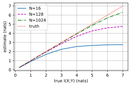
With 256 candidates, the InfoNCE lower bound is at most \ln256\approx5.5 nats.
03
Variational bounds and InfoNCE
bound it below, then maximize the bound
Bound MI from below
Variational bounds
- Barber–Agakov: a decoder, I \ge H(X)+\mathbb{E}[\log q(x\mid y)], low variance but biased down by the decoder’s gap.
- Donsker–Varadhan / MINE: I \ge \mathbb{E}_{P}[T] - \log\mathbb{E}_{Q}[e^T].
- NWJ: the same with e^{-1}\mathbb{E}_Q[e^T], unbiased for the bound but with heavy e^T tails.
All bound below; all are maximized, not measured.
Bias against variance
Estimator behavior
With exact critics on a known-MI pair: past \log N, NWJ’s batch-to-batch spread explodes (unbiased for its bound, heavy tails); DV’s log-of-average adds bias on top of the blow-up; InfoNCE stays steady but saturates at the ceiling:
true I    DV (MINE)         NWJ              InfoNCE
  0.5     0.50 +-  0.12     0.50 +-  0.12     0.50 +-  0.07
  1.0     1.01 +-  0.19     0.99 +-  0.22     1.00 +-  0.07
  2.0     1.93 +-  0.35     1.83 +-  0.97     1.94 +-  0.09
  4.0     3.79 +-  0.92     3.36 +-  1.18     3.67 +-  0.08
  6.0    23.22 +- 56.65     1.23 +- 11.74     4.61 +-  0.05
The estimators trade bias against variance.
InfoNCE: estimation as classification
Contrastive
Pick the positive among N-1 negatives: \mathcal L_{\mathrm{NCE}} is a plain softmax cross-entropy, and the estimator is the ceiling minus the loss. For any critic,
I(X;Y) \ge \hat I_{\mathrm{NCE}} = \log N - \mathcal L_{\mathrm{NCE}} \le \log N,
with optimal critic f^\star = \mathrm{pmi}+c. This is the loss of CPC, SimCLR, and CLIP.
Negative Count Caps the InfoNCE Bound
In practice
A small MLP critic at \rho=0.99 (I\approx1.96 nats): at N=2 the bound cannot clear \ln 2; widen the batch and it climbs toward the truth:
N =    2: ln N = 0.693, InfoNCE bound = 0.570 nats
N =    8: ln N = 2.079, InfoNCE bound = 1.407 nats
N =   32: ln N = 3.466, InfoNCE bound = 1.762 nats
N =  128: ln N = 4.852, InfoNCE bound = 1.888 nats
true I(X;Y) = 1.959 nats
In SimCLR and CLIP the critic is a scaled cosine, f = \mathrm{sim}(z_x,z_y)/\tau; the temperature is distillation’s knob again, concentrating the loss on the hardest negatives.
04
The bottleneck and the limits of MI
compression with a purpose, Fano, and the scope of MI estimates
The information bottleneck
Compression with a purpose
\min\; I(X;Z) - \beta\,I(Y;Z): squeeze the input, keep the label. The DPI makes it well-posed (I(Y;Z)\le I(X;Y)), and \beta sweeps the frontier; below \beta = 1/\rho^2 the code collapses to nothing.
Fano: MI floors the error rate
The guarantee
H_b(P_e) + P_e\log(k-1) \ge H(X\mid Y) = H(X) - I(X;Y). Too little MI makes low error impossible:
5% error on 1000 balanced classes needs I(X;Y) >= 6.364 nats
InfoNCE can reach that value only if N >= e^I = 581
5% error on 1000 classes demands 6.36 nats; taking the ceiling at face value, certifying that much MI needs batches of N \gtrsim e^{6.36} \approx 581. The ceiling and the floor meet.
What MI estimates establish
The caveats
Read the MI number as a capped bound; judge the objective by its representations. The calculus, the DPI, Fano’s lower bound, and the variational bounds remain valid when interpreted with their stated assumptions.
The “compression phase” of training is contested (Saxe et al.: an estimator artifact for \tanh nets). Read MI as a training signal, not a readout.
Mutual Information Measures Dependence, Not Usefulness
Wrap-up
- MI = KL from independence; three entropy forms; symmetric, \ge 0.
- Gaussian anchor -\tfrac12\log(1-\rho^2); MI catches nonlinear dependence.
- DPI: processing only loses information; invertible maps lose none.
- Histograms and KSG degrade in high dimension; distribution-free lower confidence guarantees grow at most on the order of \log N.
- InfoNCE = classification: \hat I_{\mathrm{NCE}} = \log N - \mathcal L, the loss of CPC, SimCLR, CLIP.
- IB compresses with a purpose; Fano floors the error; read MI as a signal.
Every loss in this chapter is a code length, and every divergence a choice of how to compare distributions.