Generalization

Dive into Deep Learning · §2.6

Fitting the training data is not the goal
telling memorization apart from learning · the U-curve · model selection.

Two students, one exam

The parable

Two students prepare from the same stack of past exams.

Extraordinary Ellie memorizes every answer: 100% on any question she has seen, and frozen by one she has not.
Inductive Irene can barely memorize, but picks up patterns: a steady 90%, seen or unseen.

If the exam recycles old questions, Ellie wins. If it is fresh, Irene does. Every trained model is one of these two students, and the training error alone cannot tell you which.

This section builds the instruments that can: held-out data, the generalization gap, and the bias-variance trade-off.

Two Errors

the statistic we see vs. the expectation we want

Training error vs. generalization error

Two Errors

Training error, an average over the data we have: R_\textrm{emp} = \tfrac1n \sum_{i=1}^n l\bigl(\mathbf{x}^{(i)}, y^{(i)}, f\bigr)

Generalization error, an expectation over data we will never fully see: R = E_{(\mathbf{x},y)\sim P}\bigl[\,l(\mathbf{x}, y, f)\,\bigr]

We can never compute R. We estimate it on held-out data: a fixed model on fresh samples is just mean estimation.

The IID assumption

Two Errors

Train and test are drawn independently from the identical distribution P(X,Y).

The training error is a biased gauge of R: the model was chosen using that very data, so it flatters itself.

Drop IID, let the distribution shift from P to Q, and without a further assumption nothing can be said about generalization at all.

Model Complexity

the bias-variance trade-off and the U-curve

The bias-variance trade-off

Model Complexity

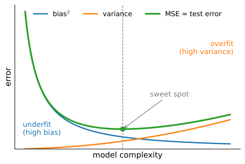
Too simple → misses the signal: high bias (underfitting).
Too flexible → chases the noise: high variance (overfitting).

Their sum, plus an irreducible noise floor, is the test error, which bottoms out at a sweet spot.

Bias falls and variance rises with complexity; their sum, plus an irreducible noise floor, is the U-shaped test error.

Reading the gap

Model Complexity

Both errors high, small gap → too simple. Underfitting; reach for more capacity.
Train error far below test → severe overfitting.

The generalization gap is R - R_\textrm{emp}.

Overfitting is not always bad: the best deep models often fit training data far better than holdout. We chase low R, and mind the gap only when it blocks us.

What makes a model complex?

Model Complexity

A model that can fit any labeling has told us nothing (Popper’s falsifiability).

Complexity is more than parameter count: it is also the range of values parameters may take. Kernel methods have infinitely many parameters yet stay controlled.

Low training error alone never certifies low generalization error, on its own it cannot rule it out either.

The Demo

fit polynomials of growing degree to a noisy cubic

Polynomial fitting is linear regression in disguise

The Demo

Predict \hat y = \sum_{i=0}^d x^i w_i: take the powers of x as features and it is plain least squares, with the degree d as a capacity dial. The rig: a degree-3 target, and only 20 training points, so high degrees have room to misbehave:

np.random.seed(0)
max_degree = 20                  # highest polynomial degree we will fit
n_train, n_test = 20, 100        # few training points, so high degrees overfit
true_w = np.zeros(max_degree)
true_w[:4] = np.array([5, 1.2, -3.4, 5.6])

x = np.random.uniform(-1, 1, size=n_train + n_test)
poly = np.power(x.reshape(-1, 1), np.arange(max_degree))   # column i holds x**i
labels = poly @ true_w + np.random.normal(scale=0.1, size=n_train + n_test)

One fit per degree, scored on both splits

The Demo

Fit the first d{+}1 power columns by least squares; record the loss on train and on 100 held-out test points.

def fit_degree(d):
    cols = slice(0, d + 1)
    w, *_ = np.linalg.lstsq(poly[:n_train, cols], labels[:n_train], rcond=None)
    err = poly[:, cols] @ w - labels
    return (err[:n_train] ** 2).mean(), (err[n_train:] ** 2).mean()

Three verdicts to predict before looking: degree 1 (too rigid), degree 3 (the truth’s own degree), degree 19 (one parameter per data point).

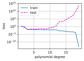
Degree 19: train error zero, test error 5 × 10¹³

The Demo · the verdict

for name, d in [('underfitting (degree 1) ', 1),
                ('just right   (degree 3) ', 3),
                ('overfitting   (degree 19)', 19)]:
    train_mse, test_mse = fit_degree(d)
    print(f'{name}: train {train_mse:8.4f}   test {test_mse:12.4f}')

underfitting (degree 1) : train   1.6698   test       1.7318
just right   (degree 3) : train   0.0136   test       0.0129
overfitting   (degree 19): train   0.0000   test 49271508224071.6328

Degree 19 fits the 20 points essentially exactly, and pays with a test error of 5\times10^{13}, fifteen orders of magnitude worse than degree 3. Zero training error certified nothing.

Sweep the degree: the U-curve, measured

The Demo · result

Train loss falls monotonically. Test loss dips to the sweet spot near degree 3, then blows up, exactly the shape the theory drew.

This is the bias-variance U-curve, now traced from real numbers rather than sketched.

The U-curve, decomposed

The Demo · payoff

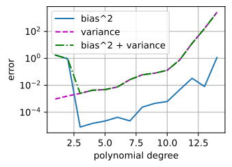
We know the noiseless target, so we can compute bias and variance: redraw the training noise 200 times, refit each degree, and measure

bias²: how far the average fit is from the truth;
variance: how much the fit fluctuates across draws.

Bias collapses once the model class contains the truth (degree 3); variance grows relentlessly with surplus capacity. Their sum bottoms out exactly at the sweet spot.

More data, more room

The Demo

Fix the model: fewer samples means more, and more severe, overfitting.

So complexity should grow with data, not ahead of it. Deep nets beat linear models only once there are many thousands of examples, which is why big datasets fuelled their rise.

Model Selection

keep the test set honest with a validation split

Never select on the test set

Model Selection

Touch the test data to choose a model and you overfit it silently, and unlike training data, nothing is left to catch you.

So split three ways: train, validation (for model selection), test (touched once). Most “test” accuracy in practice is really validation accuracy.

K-fold cross-validation

Model Selection

When data is too scarce to spare a validation set: split into K folds, train on K{-}1, validate on the held-out one, rotate, and average the K scores.

Choosing K trades bias, variance, and compute: each fold trains on (K{-}1)/K of the data. If performance improves monotonically with more data, the estimate is pessimistic relative to the final full-data fit. Larger K narrows that gap but costs more fits and uses nearly identical, correlated training sets. K = 5 or 10 is a common compromise.

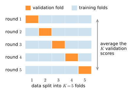
Each of the K folds serves once as the validation set; average the K validation scores.

A Modern Twist

when more capacity helps again

Double descent

A Modern Twist

The classical U is only half the story for huge models. Once capacity is large enough to interpolate the data, pushing it further often makes test error fall again.

The generalization-in-deep-learning section takes up the modern story; the concentration-and-generalization section reproduces this curve from scratch and explains the peak.

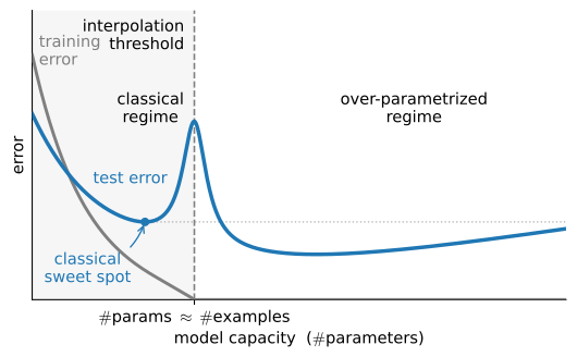
Past the interpolation threshold, test error descends a second time, the over-parametrized regime of deep learning.

Rules of thumb

Wrap-up

Generalization, not training fit, is the goal: mind the gap R - R_\textrm{emp}.
Zero training error certifies nothing: degree 19 fit 20 points exactly and tested at 5\times10^{13}.
Bias-variance: bias² falls, variance rises; their sum (plus a noise floor) is the test-error U-curve, and we computed both.

Select models with a validation set or K-fold CV (K=5–10), never the test set.
More data rarely hurts; let complexity grow with it, not ahead of it.
All of this rests on IID, and huge models can defy the classical U via double descent.